Lab 5: Power

Fabio Setti

PSYC 6802 - Introduction to Psychology Statistics

Today’s Packages and Data 🤗

install.packages("pwr")

library(pwr)

• pwr

The pwr package (Champely et al., 2020) includes functions to conduct power analysis for some statistical analyses and experimental designs. Click here for examples on all the types of power calculations that the package allows for.

Data

We won’t look at data too much today, but let’s load the data from last lab, which will come up for retrospective power analysis.

dat <- rio::import("https://fabio-setti.netlify.app/data/Cuisine_rating.csv")

What is Power⚡?

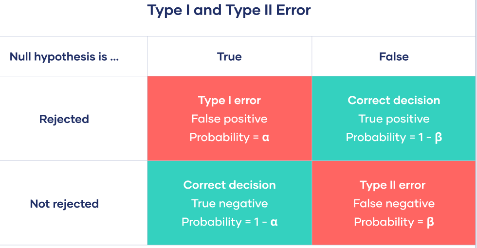
Power: Statistical power is defined as the probability of correctly rejecting the null hypothesis if \(H_0\) is false. Power is also known as 1 - Type II error rate. Type II error rate is denoted with \(\beta\), and is the probability of failing to reject a false \(H_0\).

In practice, power is used is mostly to answer the question: “how big of a sample size do I need to get a p-value lower than .05 given a certain effect size?” (pretty useless question if you ask me 😑)

The probability of making a Type I error is always the level of significance, \(\alpha\). As you know, the level of significance is almost unilaterally \(.05\). So, unless specified otherwise, \(\alpha = .05\).

On the other hand, it is common to generally look for a sample size that gives a power of \(\beta = .8\). This would mean that if \(H_0\) is false, you would reject it \(80\%\) of the times.

The Logic of the pwr Functions

All of the functions in the pwr package work in very similar fashion. They will generally include arguments representing these 4 factors that influence power:

• Effect size: could be \(d\) in the case of a \(t\)-test, \(W\) for a \(\chi^2\) test, \(R^2\) for regression…
• Sample size: How many participants you expect to have/will need. Will usually be the n = argument.
• Type I error rate: This is the desired \(\alpha\) level. This is always the sig.level = argument.
• Power: The desired power. This is always the power = argument.

The pwr functions will expect to leave one of these 4 arguments empty (= NULL), and will return its value

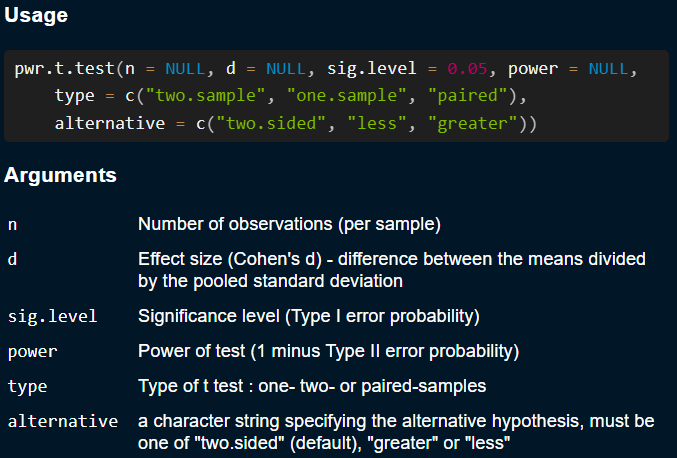
As an example, this is the pwr.t.test() Function

These arguments may be named differently depending on the type of power analysis, so always check the function help menu when trying to use any of the pwr package functions.

Power For χ² Tests

Let’s say the we want to run a study where we want to evaluate the effecicacy of a new cancer treatment versus an old one by checking whether there is an association between type of treatment and cancer remission.

We want to find out the necessary sample size (\(N\)) required to:

1. Achieve \(.8\) power,
2. At \(\alpha = .05\),
3. given that we expect an effect of \(W = .5\).

Furthermore, we know that \(df = 1\) because we would have a \(2 \times 2\) table (new/old treatment VS remission/ no remission).

Given the desired power, \(\alpha\) level, and expected effect size, we would need \(N = 32\) participants (you always round up!)

pwr.chisq.test(w = .5, 
               N = NULL, 
               df = 1, 
               sig.level = .05, 
               power = .8)

     Chi squared power calculation 

              w = 0.5
              N = 31.39544
             df = 1
      sig.level = 0.05
          power = 0.8

NOTE: N is the number of observations

Retrospective Power Analysis

Sometimes it is insightful to check how much power a study had given the observed effect size. If you remember the airplane delays example from Lab 3, We got the following results:

1. At \(\alpha = .05\),
2. with \(N = 106596\) observations,
3. we got an effect of roughly \(W = .06\),
4. And we had \(df = 1\).

How much power did we have? (probability to reject \(H_0\))

We had power \(= 1\). This comes as no surpise given the huge sample size, which is by far the most impactful thing on power.

This means that given a large enough sample size, anything becomes significant 🤷

pwr.chisq.test(w = .06, 
               N = 106596, 
               df = 1, 
               sig.level = .05, 
               power = NULL)

     Chi squared power calculation 

              w = 0.06
              N = 106596
             df = 1
      sig.level = 0.05
          power = 1

NOTE: N is the number of observations

Power for One Sample \(t\)-tests

In Lab 4 we ran a one sample t-test to test whether average restaurant ratings were significantly different from 3. with \(d\) = .21 and \(N\) = 200 we can do a retrospective power calculation:

pwr.t.test(n = 200,
           d = .21,
           sig.level = .05,
           power = NULL,
           type = "one.sample")

     One-sample t test power calculation 

              n = 200
              d = 0.21
      sig.level = 0.05
          power = 0.8402593
    alternative = two.sided

So, given the observed results, we had \(84\%\) power.

Alternatively, let’s say that we want \(95 \%\) power under the same conditions; how large of a sample size do we need? Then, ⇒ ⇒

We would need \(N = 297\) participants.

pwr.t.test(n = NULL,
           d = .21,
           sig.level = .05,
           power = .95,
           type = "one.sample")

     One-sample t test power calculation 

              n = 296.5928
              d = 0.21
      sig.level = 0.05
          power = 0.95
    alternative = two.sided

Power for Independent Sample \(t\)-tests

In Lab 4, we tested whether males and females were significantly different on average food rating.

t.test(Overall_Rating ~ Gender, 
       data = dat)

    Welch Two Sample t-test

data:  Overall_Rating by Gender
t = 1.1696, df = 154.21, p-value = 0.244
alternative hypothesis: true difference in means between group Female and group Male is not equal to 0
95 percent confidence interval:
 -0.1288966  0.5030181
sample estimates:
mean in group Female   mean in group Male 
            3.335366             3.148305 

library(effectsize)
cohens_d(Overall_Rating ~ Gender, 
         data = dat,
         pooled_sd = FALSE)

Cohen's d |        95% CI
-------------------------
0.17      | [-0.12, 0.46]

- Estimated using un-pooled SD.

And we will also need the sample size for both groups:

table(dat$Gender)

Female   Male 
    82    118 

How much power did we have?

pwr.t2n.test(n1 = 82, n2 = 117,
             d = 0.15, 
             sig.level = 0.05,
             power = NULL)

     t test power calculation 

             n1 = 82
             n2 = 117
              d = 0.15
      sig.level = 0.05
          power = 0.1792332
    alternative = two.sided

Only \(18\%\) power. It means that it was fairly unlikely for us to reject \(H_0\) given the observed effect size and sample size.

Low Power is bad Because…

Low power is not bad because it will be hard to get \(p < .05\). Low power is bad because when you do get \(p < .05\) with low power, it is likely that:

1. The effect size will be largely overestimated! (Type M error).
2. The effect will be in the wrong direction! (Type S error).

You may have been “lucky” in the sense that your result was significant, but it will likely not replicate in future research. Your “lucky” result is ultimately a bad thing for the field (!!). And you will not see the results of many other people who ran the same analysis but did not get a significant p-value (publication bias!).

So, I think people care about power for the wrong reasons 🤷 Some related blog posts/manuscripts by Andrew Gelman:

• 80% power is a lie and NIH grants
• You don’t have 80% Power
• You calculate power based on biased literature
• Type I and Type II error rates do not exist

Andrew Gelman, Columbia professor and very opinionated man. I like his opinions.

Appendix: Power For F-tests, Correlation, and Regression

Power for Correlation

Power for correaltion coefficients is fairly streightforward to compute.

• If we expect to see \(r =.3\), what sample size do we need to have \(80\%\) power at \(\alpha = .05\)?

# we'll need 85 participants (you round up n)
pwr.r.test(r = .3,
           sig.level = .05,
           power = .8)

     approximate correlation power calculation (arctangh transformation) 

              n = 84.07364
              r = 0.3
      sig.level = 0.05
          power = 0.8
    alternative = two.sided

• How much power do we have if \(r =.2\), and \(N = 75\) at \(\alpha = .05\)?

# around .41 (41%) power
pwr.r.test(r = .2,
           sig.level = .05,
           n = 75)

     approximate correlation power calculation (arctangh transformation) 

              n = 75
              r = 0.2
      sig.level = 0.05
          power = 0.4091307
    alternative = two.sided

Power in Regression

In regression, We calculate power based on \(R^2\). More specifically, we use Cohen’s \(f^2\). there are two slight variations on \(f^2\):

When you have a single set of predictors and you want to calculate power for a regression,

\[ f^2 = \frac{R^2}{1 - R^2} \]

When you want to calculate power for \(\Delta R^2\) (see this), whether a set of predictors B provides a significant improvement over an original set of predictors A,

\[ f^2 = \frac{R^2_{AB} - R^2_{A}}{1 - R^2_{AB}} \]

Where \(R^2_{AB} - R^2_{A} = \Delta R^2\), the improvement of adding the set of predictors B.

Larger \(R^2\) value imply larger \(f^2\) values. Some guidelines are that \(f^2\) of .02, .15, and .35 can be interpreted as small, medium, and large effect sizes respectively. Why do we use \(f^2\)? Check out the this if you are curios!

Power For \(R^2\)

Let’s say that we hypothesize that depression (\(X_1\)), anxiety (\(X_2\)), and social support (\(X_3\)) should predict willingness to partake in novel social experiences (\(Y\)). We look at the literature and we expect our variables to jointly explain \(15\%\) (i.e., \(R^2 = .15\)) of the variance in willingness to partake in novel social experiences. How many participants do we need to collect to get \(80\%\) power?

Fist we need to calculate \(f^2\):

(f2 <- .15/(1-.15))

[1] 0.1764706

u stands for \(\mathrm{df_1}\) and v stands for the \(\mathrm{df_2}\) of the \(F\)-distribution. We know from Lab 4 that \(\mathrm{df_2} = n - \mathrm{df_1} - 1\). Thus,

\[ n = \mathrm{df_2} + 1 + \mathrm{df_1} = 61.18 + 1 + 3 = 65.18 \]

We need \(66\) participants (you always round up!) to achieve \(80\%\) power.

Then, we can use the pwr.f2.test() function from the pwr package

pwr::pwr.f2.test(u = 3,  f2 = f2, 
                 sig.level = 0.05, power = 0.8)

     Multiple regression power calculation 

              u = 3
              v = 61.8227
             f2 = 0.1764706
      sig.level = 0.05
          power = 0.8

Power For \(\Delta R^2\)

We further hypothesize that if we add openness to experience (\(X_4\)) to our model, we will explain an additional \(5\%\) (\(\Delta R^2 = .05\)) of variance in willingness to partake in novel social experiences (\(Y\)). Originally, we specified \(R^2 = .15\), so after adding \(X_4\), we expect \(R^2 = .2\).

We use the second formula from 2 slides ago to get \(f^2\):

(f2 <- .05/(1-.20))

[1] 0.0625

u is going to be \(1\) because we only have 1 additional predictor, \(X_4\):

pwr::pwr.f2.test(u = 1,  f2 = f2, 
                 sig.level = 0.05, power = 0.8)

     Multiple regression power calculation 

              u = 1
              v = 125.5312
             f2 = 0.0625
      sig.level = 0.05
          power = 0.8

So, if we want to have \(80\%\) power for \(\Delta R^2 = .05\), we now need at least \(131\) participants. We know this because

\[ n = 125.5 + 4 + 1 = 130.5 \]

where \(4\) is the number of predictors in the full regression after adding \(X_4\).

I already linked this in the first slide, but this page has very detailed explanations on how to use all the functions from the pwr package.

References

Champely, S., Ekstrom, C., Dalgaard, P., Gill, J., Weibelzahl, S., Anandkumar, A., Ford, C., Volcic, R., & Rosario, H. D. (2020). Pwr: Basic Functions for Power Analysis.