Lab 6: Multicollinearity, Dominance Analysis, and Power
PSYC 7804 - Regression with Lab
Fabio Setti
Spring 2025
Today’s Packages and Data 🤗
The dominanceanalysis package (Navarrete & Soares, 2024) contains functions to run dominance analysis in R.
The pwr package (Champely et al., 2020) includes functions to conduct power analysis for some statistical analyses and experimental designs. Click here for examples on all the types of power calculations that the package allows for.
Background About the data
I am using some of the data from Setti & Kahn (2024), where (yes I am citing myself, but it makes sense for this lab, I promise 😶🫣) we looked at how facets of openness to experience (both from the big five and the HEXACO) predict music preference.
For the data here I selected only 3 personality facets and 1 dimension of music preference.
- Intense: Preference for the intense music dimension, which includes genres such as rock, punk, metal.
- Advnt: Adventurousness facet of big 5 openness to experience.
- Intel: Intellect facet of big 5 openness to experience.
- Uncon: Unconventionality facet of HEXACO openness to experience.
Higher values mean higher preference/levels of personality trait
Dimensions of Music Preference 🎶
Rentfrow & Gosling (2003) was a seminal study in the field of music preference, where it was found that preference for music genres cluster together (e.g., if you like punk music, you tend to like metal music). Later Rentfrow et al. (2011) proposed a 5-factor structure of music preference: sophisticated (e.g., classical, blues, jazz), unpretentious (e.g., country and folk), intense (e.g, rock, punk, metal), mellow (e.g., pop, electronic), and contemporary (e.g., rap, RnB). This 5-factor structure seems to work fairly well, although I would suspect that 1 or 2 more factors would emerge with a more comprehensive selection of music genres.
This data fits the lab topic well because in the paper we had to figure out a way of dealing with high multicollinearity, and dominance analysis ended up helping a lot!
Regression coefficients Weirdness
It is common practice to add covariates to regression models without giving it much thought (adding a covariate simply means adding additional predictors). However, some strange things 👽 may happen if you add variables too casually to regression models.
For now, let’s see how Adventurousness and intellect relate preference for Intense music:
        Intense Advnt Intel
Intense    1.00  0.24  0.27
Advnt      0.24  1.00  0.96
Intel      0.27  0.96  1.00
The correlations are all positive.
But wait, the relation between
Advnt and Intense becomes negative after accounting for Intel 🙀
Let’s say we want to know the relation between
Advnt and Intense while accounting for Intel. We run a multiple regression:
Coefficients:
            Estimate Std. Error t value Pr(>|t|)
(Intercept)  -2.3076     0.4642  -4.972 1.02e-06 ***
Advnt        -0.6444     0.4520  -1.426   0.1548
Intel         1.2766     0.4571   2.793   0.0055 **
---
Signif. codes:  0 '***' 0.001 '**' 0.01 '*' 0.05 '.' 0.1 ' ' 1

Residual standard deviation: 0.9686 on 366 degrees of freedom
Multiple R-squared: 0.07685
F-statistic: 15.23 on 2 and 366 DF,  p-value: 4.416e-07
    AIC     BIC
1028.61 1044.26
Visualizing Multicollinearity
When strange things happen, visualizing your data (if possible) is always a good idea.
One apparent issue is that
Advnt and Intel are extremely correlated (\(r = .96\)). You can see it from the 3D plot, which is essentially a 2D plot (Advnt and Intel are effectively a single variable, not two separate ones). This is a case of multicollinearity.
We are asking for a 3D plane when we should just ask for a line. In such cases, strange things are bound to happen.
Back to Semi-Partial Correlations
If you remember, semi-partial correlations calculate the correlation between \(y\) and \(x\) after removing the explained variance of \(z\) from only one variable.
$estimate
            Intense      Advnt     Intel
Intense  1.00000000 -0.0715963 0.1402480
Advnt   -0.01976479  1.0000000 0.9340608
Intel    0.03841693  0.9268286 1.0000000
We want to look at the first row. We can see that the relation between Intense and advnt is negative after the variance explained by Intel is taken out of Advnt.
As we saw a few slides back, by themselves both variables are positively correlated with Intense
  Intense     Advnt     Intel
1.0000000 0.2391202 0.2678095
A Word of Advice
When the sign of correlations and semi-partial correlations are different, something strange is happening. Multicollinearity may be the reason, but other possibilities exist (see here).
Variance Inflation Factor
Probably the quickest way to check for multicollinearity is to calculate the variance inflation factor (VIF) for each predictor. For a predictor \(x\), the formula is:
\[VIF_x = \frac{1}{1 - R^2}\]
Importantly, the \(R^2\) in the VIF formula stands for the variance explained in the predictor \(x\) by all other predictors.
Another Perspective: Residuals
As shown in Lab 4, regression coefficients are calculated based on the residuals of the predictors after controlling for all other predictors. But, if Advnt and Intel are so correlated, what happens to their residual after controlling fo one another?
The residuals have almost no variance left! If a variable has variance of 0, it is always the same number (i.e., a constant), and cannot predict anything. A consequence of multicollinearity is that the regression coefficients that are calculated based on these residuals should not be interpreted.
However, \(R^2\) is untouched by multicollinearity! So, you can still interpret \(R^2\) just fine with high multicollinearity.
Dominance Analysis
Dominance analysis (Azen & Budescu, 2003; Budescu, 1993) main application is to determine the relative importance of a set of predictor variables. DA provides a way of ranking predictors by importance.
Let’s say we have three predictors, \(x_1\), \(x_2\) and \(x_3\). We want know which one is the most important relative to the other 2 predictors. DA looks at how much each variable adds to \(R^2\) when it is added to all possible regression subsets.
For Example, for \(x_1\), we would look at how much the \(R^2\) increases when we add it to a regression (1) with no variables , (2) only with \(x_2\), (3) only with \(x_3\), and (4) with \(x_2\) and \(x_3\).
Different dominance patterns (complete dominance, conditional dominance, general dominance) between variables can be established depending on the results of DA.

Example with our Data
In the case of our data we have 3 facets of openness to experience: adventurousness, intellect, and unconventionality. We want to know how these three variables is the most important in predicting preference for Intense music.
* Fit index:  r2

Average contribution of each variable:

Uncon Intel Advnt
0.064 0.034 0.023

Dominance Analysis matrix:
             model level   fit Advnt Intel Uncon
                 1     0     0 0.057 0.072 0.098
             Advnt     1 0.057        0.02 0.054
             Intel     1 0.072 0.005       0.045
             Uncon     1 0.098 0.013  0.02
   Average level 1     1       0.009  0.02 0.049
       Advnt+Intel     2 0.077             0.044
       Advnt+Uncon     2 0.111       0.011
       Intel+Uncon     2 0.117 0.004
   Average level 2     2       0.004 0.011 0.044
Advnt+Intel+Uncon 3 0.121 -
model: variables in the regression. -
level: number of variables in the regression. -
fit: \(R^2\) value for given regression. -
remaining columns: contribution in \(R^2\) when adding variable in column.
let’s go over the meaning of the columns in the output
We see that across all possible regressions,
Uncon contributes the most \(R^2\) on average, \(.064\) (i.e., general dominance).
Additional Dominance Patterns
So, on average Uncon is the most important predictor or preference for Intense music. This is just on average across all possible regression. We can build dominance matrices with j rows and i columns.
A dominance matrix will contain a 1 if the variable in the row \(j\) dominates the one in column \(i\). You will see a .5 if the dominance pattern between two variables cannot be established.
In both cases, Uncon dominates the other two variables. We now have a really strong case to claim that Uncon is the most important predictor of preference for Intense music among our 3 openness facets.
Uncertainty and Inference in DA
As it is the case with any statistical procedure, our results are based on a sample, and there is uncertainty about our results (e.g., are they due to sampling error?). We can use bootstrap to check how often the dominance pattern replicates across every bootstrap sample (1000 in this case):
Dominance Analysis
==================
Fit index: r2
   dominance     i     k Dij  mDij SE.Dij   Pij   Pji Pnoij   Rep
    complete Advnt Intel   0 0.032  0.155 0.018 0.954 0.028 0.954
    complete Advnt Uncon   0 0.072  0.193 0.013 0.869 0.118 0.869
    complete Intel Uncon   0 0.159  0.301 0.073 0.756 0.171 0.756
 conditional Advnt Intel   0 0.032  0.155 0.018 0.954 0.028 0.954
 conditional Advnt Uncon   0 0.072  0.193 0.013 0.869 0.118 0.869
 conditional Intel Uncon   0 0.159  0.301 0.073 0.756 0.171 0.756
     general Advnt Intel   0 0.022  0.147 0.022 0.978 0.000 0.978
     general Advnt Uncon   0 0.052  0.222 0.052 0.948 0.000 0.948
     general Intel Uncon   0 0.148  0.355 0.148 0.852 0.000 0.852
Skipping over some stuff, the column that we care most about is the rep column.
This column shows the proportion of bootstrap samples where the dominance pattern in the row was replicated. In general, Uncon seems to fairly consistently dominate all other variables.
DA and Multicollinearity
If you remember \(R^2\) is unaffected by multicollinearity. By extension, DA is unaffected too, as it only deals with \(R^2\). Thus, DA can be a good way of making inferences about your variables when your regression coefficients are not interpretable due to high multicollinearity (which is why it came up in my case!)
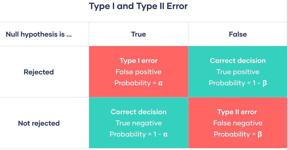
What is Power⚡?
Power: Statistical power is defined as the probability of correctly rejecting the null hypothesis if \(H_0\) is false. Power is also known as 1 - Type II error rate. Type II error rate is denoted with \(\beta\), and is the probability of failing to reject a false \(H_0\).
In practice, power is used is mostly to answer the question: “how big of a sample size do I need to get a p-value lower than .05 given a certain effect size?” (not the most useful question if you ask me)
The probability of making a Type I error is always the level of significance, \(\alpha\). As you know, the level of significance is almost unilaterally \(.05\). So, unless specified otherwise, \(\alpha = .05\).
On the other hand, it is common to generally look for a sample size that gives a power of \(\beta = .8\). This would mean that if \(H_0\) is false, you would reject it \(80\%\) of the times.
Power for Correlation
Calculating power for correlation, \(r\), is fairly straightforward. In general calculating power involves these pieces of information:
The effect size. Could be \(r\), \(d\), \(f^2\), …
The significance level, \(\alpha\)
The power, \(1 - \beta\)
The sample size, \(N\)
Most power software will provide any of these elements given the remaining ones. the
pwr package works in the same way.
- If we expect to see \(r =.3\), what sample size do we need to have \(80\%\) power at \(\alpha = .05\)?
Power in Regression
In regression, We calculate power based on \(R^2\). More specifically, we use Cohen’s \(f^2\). there are two slight variations on \(f^2\):
When you have a single set of predictors and you want to calculate power for a regression,
\[ f^2 = \frac{R^2}{1 - R^2} \]
When you want to calculate power for \(\Delta R^2\) (see Lab 6), whether a set of predictors B provides a significant improvement over an original set of predictors A,
\[ f^2 = \frac{R^2_{AB} - R^2_{A}}{1 - R^2_{AB}} \] Where \(R^2_{AB} - R^2_{A} = \Delta R^2\), the improvement of adding the set of predictors B.
Larger \(R^2\) value imply larger \(f^2\) values. Some guidelines are that \(f^2\) of .02, .15, and .35 can be interpreted as small, medium, and large effect sizes respectively. Why do we use \(f^2\)? Check out the appendix if you are curios!
Power For \(R^2\)
Let’s say that we hypothesize that depression (\(X_1\)), anxiety (\(X_2\)), and social support (\(X_3\)) should predict willingness to partake in novel social experiences (\(Y\)). We look at the literature and we expect our variables to jointly explain \(15\%\) (i.e., \(R^2 = .15\)) of the variance in willingness to partake in novel social experiences. How many participants do we need to collect to get \(80\%\) power?
u stands for \(\mathrm{df_1}\) and v stands for the \(\mathrm{df_2}\) of the \(F\)-distribution. We know from Lab 4 that \(\mathrm{df_2} = n - \mathrm{df_1} - 1\). Thus,
\[ n = \mathrm{df_2} + 1 + \mathrm{df_1} = 61.18 + 1 + 3 = 65.18 \]
We need \(66\) participants (you always round up!) to achieve \(80\%\) power.
Power For \(\Delta R^2\)
We further hypothesize that if we add openness to experience (\(X_4\)) to our model, we will explain an additional \(5\%\) (\(\Delta R^2 = .05\)) of variance in willingness to partake in novel social experiences (\(Y\)). Originally, we specified \(R^2 = .15\), so after adding \(X_4\), we expect \(R^2 = .2\).
So, if we want to have \(80\%\) power for \(\Delta R^2 = .05\), we now need at least \(131\) participants. We know this because
\[ n = 125.5 + 4 + 1 = 130.5 \]
where \(4\) is the number of predictors in the full regression after adding \(X_4\).
I already linked this in the first slide, but this page has very detailed explanations on how to use all the functions from the pwr package.
What about power for Slopes?
Calculating power for regression slopes is very tricky. This is because power for a single regression slope depends on its standard error. The standard error formula for a slope in a regression with two predictors is:
\[ \mathrm{SE}_{b_1} = \frac{S_Y}{S_{X_1}}\sqrt{\frac{1 - r_{Y\hat{Y}}}{n - p - 1}}\times\sqrt{\frac{1}{1 - r^2_{12}}} \]
The equation itself is not super important to know. But there are some useful things to know:
The one thing to keep in mind is that the smaller \(\mathrm{SE}_{b_1}\), the higher your power. \(n\), the sample size, is in the denominator, meaning that larger sample size decreases \(\mathrm{SE}_{b_1}\)…so, more \(n\), more power 😀.
The part that makes it tricky is the \(\sqrt{\frac{1}{1 - r^2_{12}}}\). This is the VIF that we saw a few slides back. Since the VIF multiplies the rest of the equation, larger VIF increases \(\mathrm{SE}_{b_1}\), thus reducing power. The VIF depends on the correlation of a predictor with all the other predictors, which is really hard to guess.
Suggestion: If you want to do power analysis for a single regression coefficient, you should frame it in terms of how much \(\Delta R^2\) you think that coefficient will produce once you add it to the regression. This is equivalent to what we did on the previous slide actually!
Low Power is bad Because…
Low power is not bad because it will be hard to get \(p < .05\). Low power is bad because when you do get \(p < .05\) with low power, it is likely that:
- The regression coefficients will be largely overestimated! (Type M error).
- The sign of some regression coefficients will be in the wrong direction! (Type S error).
You may have been “lucky” in the sense that your result was significant, but it will likely not replicate in future research. Your “lucky” result is ultimately a bad thing for the field (!!). And you will not see the results of many other people who ran the same analysis but did not get a significant p-value (publication bias!).
So, I think people care about power for the wrong reasons 🤷 Some related blog posts/manuscripts by Andrew Gelman:

References
Azen, R., & Budescu, D. V. (2003). The dominance analysis approach for comparing predictors in multiple regression. Psychological Methods, 8(2), 129–148. https://doi.org/10.1037/1082-989X.8.2.129
Budescu, D. V. (1993). Dominance analysis: A new approach to the problem of relative importance of predictors in multiple regression. Psychological Bulletin, 114(3), 542–551. https://doi.org/10.1037/0033-2909.114.3.542
Champely, S., Ekstrom, C., Dalgaard, P., Gill, J., Weibelzahl, S., Anandkumar, A., Ford, C., Volcic, R., & Rosario, H. D. (2020). Pwr: Basic Functions for Power Analysis.
Cohen, J. (1988). Statistical Power Analysis for the Behavioral Sciences (2nd edition). Routledge.
Fox, J., Weisberg, S., Price, B., Adler, D., Bates, D., Baud-Bovy, G., Bolker, B., Ellison, S., Firth, D., Friendly, M., Gorjanc, G., Graves, S., Heiberger, R., Krivitsky, P., Laboissiere, R., Maechler, M., Monette, G., Murdoch, D., Nilsson, H., … R-Core. (2024). Car: Companion to Applied Regression.
Navarrete, C. B., & Soares, F. C. (2024). Dominanceanalysis: Dominance Analysis.
Rentfrow, P. J., Goldberg, L. R., & Levitin, D. J. (2011). The structure of musical preferences: A five-factor model. Journal of Personality and Social Psychology, 100(6), 1139–1157. https://doi.org/10.1037/a0022406
Rentfrow, P. J., & Gosling, S. D. (2003). The do re mi’s of everyday life: The structure and personality correlates of music preferences. Journal of Personality and Social Psychology, 84(6), 1236–1256. https://doi.org/10.1037/0022-3514.84.6.1236
Setti, F., & Kahn, J. H. (2024). Evaluating how facets of openness to experience predict music preference. Musicae Scientiae, 28(1), 143–158. https://doi.org/10.1177/10298649231174751
Wickham, H., & RStudio. (2023). Tidyverse: Easily Install and Load the ’Tidyverse’.
Appendix: Why \(f^2\)? The non-central \(F\)-distribution
\(f^2\) and non-central \(F\)-distribution
We know that \(R^2\) is itself a measure of effect size; so why do we calculate \(f^2\) to compute power? Chapter 9 of good old Cohen (1988) goes in more detail, but \(f^2\) is more general and convenient than \(R^2\).
Power for \(F\)-tests is calculated by comparing two things:
- The null \(F\)-distribution if \(R^2 = 0\). This is a normal \(F\)-distribution with \(\mathrm{df_1} = k\) and \(\mathrm{df_2} = n - k-1\).
- The \(F\)-distribution if \(R^2 \neq 0\). This is an \(F\)-distribution with \(\mathrm{df_1} = k\), \(\mathrm{df_2} = n - k-1\), and a non-centrality parameter that we will call \(L\) (in Cohen (1988), this is referred to as \(\lambda\)).
The formula to calculate \(L\) is very straightforward once we have \(f^2\):
\[ L = f^2\times(\mathrm{df_1} + \mathrm{df_2} + 1) = f^2 \times n \]
Note that the sample size, \(n\), is included in this formula, and we can solve for it such that \(n = \frac{L}{f^2}\) (neat).
The Non-central F-distribution
If \(L = f^2 \times n\), then larger \(L\) values imply either larger \(f^2\) values, larger \(n\) values, or both.
but if \(f^2 = 0\) (meaning that \(R^2 = 0\)), then \(L = 0\). When \(L = 0\), we have a normal \(F\)-distribution.
You will see that increasing \(L\) will shift the distribution to the right, making higher \(F\)-values more likely.
Power analysis for \(F\)-test finds the critical \(F\)-value when \(L = 0\), and checks how likely it is to get a higher \(F\)-value when \(L = f^2 \times n\).
Power by hand
Let’s go back to the example from some slides ago, but let’s pretend that we already ran the study with \(n = 100\), 3 predictors (\(k = 3\)), and we found a significant \(R^2 = .15\) at \(\alpha = .05\). How much power did we have?
First, we need to find the \(F\)-value from the null distribution after which everything is significant at \(\alpha = .05\). We have \(\mathrm{df_1} = 3\) and \(\mathrm{df_2} = 100 - 3 -1 = 96\):
Any \(F\)-value larger than this is going to be significant
Now, we can check how likely it is to get an \(F\)-value greater than our critical value from a non-central \(F\)-distribution where \(f^2 = \frac{.15}{1 - .15} \approx .176\). The non-centrality parameter will be \(L = .176 \times 100 \approx 17.6\)
So, in retrospect, we had roughly a \(.95\) power. That is, we had a \(95\%\) chance of getting \(p < .05\) given our sample size, number of variables, and observed \(R^2\).
oh, and because \(n = \mathrm{df_1} + \mathrm{df_2} + 1\), you can do some algebra on the \(L = f^2 \times n\) equation to find any of the other terms if you want.
Checking with the pwr.f2.test() function
As always, I want to check that the result I got is also what you would get with another function. Let’s use the pwr.f2.test():
What I just did is a general good practice. If you think you understand something but you are not \(100\%\) sure and you can use R to run the math by hand, try it! You will gain insight in the process and solidify your knowledge.
Now I know with really high certainty that my understanding of the process is accurate.
PSYC 7804 - Lab 6: Multicollinearity, Dominance Analysis, and Power