Lab 5: Added Variable Plots and Bootstrapping

PSYC 7804 - Regression with Lab

Fabio Setti

Spring 2025

Today’s Packages and Data 🤗

Data

Let’s continue with the example from Lab 4

WH_2024 <- rio::import("https://github.com/quinix45/PSYC-7804-Regression-Lab-Slides/raw/refs/heads/main/Slides%20Files/Data/World_happiness_2024.csv")

# let's peak at our variables
str(WH_2024, vec.len = 2)

'data.frame':   140 obs. of  9 variables:
 $ Country_name           : chr  "Finland" "Denmark" ...
 $ Region                 : chr  "Western Europe" "Western Europe" ...
 $ Happiness_score        : num  7.74 7.58 ...
 $ Log_GDP                : num  1.84 1.91 ...
 $ Social_support         : num  1.57 1.52 ...
 $ Healthy_life_expectancy: num  0.695 0.699 0.718 0.724 0.74 ...
 $ Freedom                : num  0.859 0.823 0.819 0.838 0.641 ...
 $ Generosity             : num  0.142 0.204 0.258 0.221 0.153 ...
 $ Corruption             : num  0.454 0.452 0.818 0.476 0.807 ...

# get the variable we are using in a single object
# not needed, but makes things cleaner

reg_vars <- WH_2024[, c("Happiness_score",
                        "Log_GDP",
                        "Freedom")]

And let’s load good old tidyverse

library(tidyverse)
theme_set(theme_classic(base_size = 16, 
                        base_family = 'serif'))

Partial regression coefficients

In Lab 4 , we used Log_GDP and Freedom to predict Happiness_score. We observed that the results were very different when we use both variables together compared to when we look at them separately

The intercept and slopes with both predictors in the model

reg_full <- lm(Happiness_score ~ Log_GDP + Freedom, 
          reg_vars)

coef(reg_full)

(Intercept)     Log_GDP     Freedom 
   1.437184    1.682053    2.859202 

The intercept and slopes with separate models with one predictor are quite different

reg_free <- lm(Happiness_score ~ Freedom, 
              reg_vars)
coef(reg_free)

(Intercept)     Freedom 
   2.623351    4.684888 

reg_GDP <- lm(Happiness_score ~ Log_GDP, 
              reg_vars)
coef(reg_GDP)

(Intercept)     Log_GDP 
   2.586466    2.135488 

The catch is that the model that includes both predictors calculates partial regression coefficients.

Calculate partial regression coefficients “By Hand”

Personally, the concept of partial regression coefficients starts making sense once I “compute” them myself and see what is going on behind the scenes.

Partial regression coefficient for Log_GDP

resid_happy_Free <- residuals(lm(Happiness_score ~ Freedom, 
               reg_vars))

resid_GDP <- residuals(lm(Log_GDP ~ Freedom, 
              reg_vars))

# the 0 + takes out the intercept, which is exactly 0 anyway in this case 
coef(lm(resid_happy_Free ~ 0 + resid_GDP))

resid_GDP 
 1.682053 

Partial regression coefficient for Freedom

resid_happy_GDP <- residuals(lm(Happiness_score ~ Log_GDP, 
               reg_vars))

resid_Free <- residuals(lm(Freedom ~ Log_GDP, 
              reg_vars))

# the 0 + takes out the intercept, which is exactly 0 anyway in this case 
coef(lm(resid_happy_GDP ~ 0 + resid_Free))

resid_Free 
  2.859202 

So, when you run multiple regression, all your slopes are calculated based on the residuals after accounting for all the other variables in the model.

Added variable plots

Then, added variables plots are simply plots between the residuals of one the predictors and \(Y\) that result by taking out the variance explained by all the other variables.

ggplot() +
  geom_point(aes(y = resid_happy_Free, 
                 x = resid_GDP))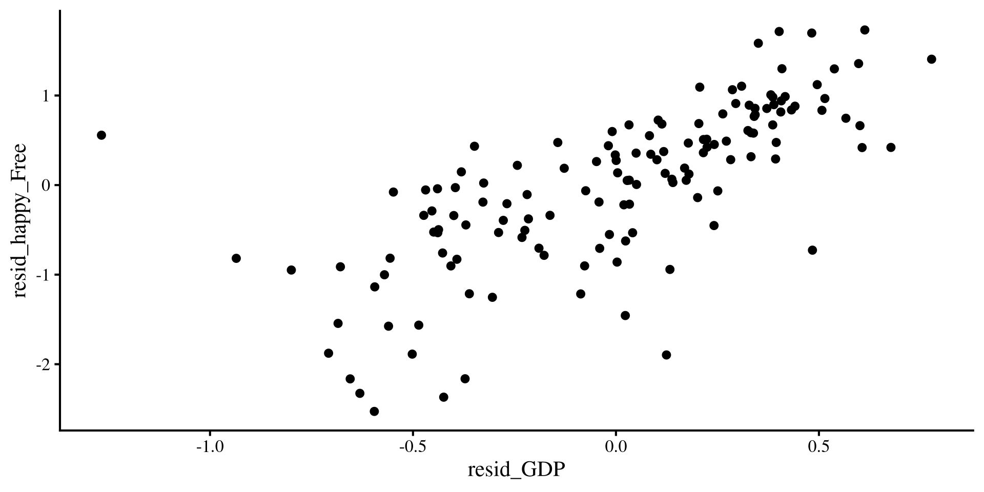

ggplot() +
  geom_point(aes(y = resid_happy_GDP, 
                 x = resid_Free))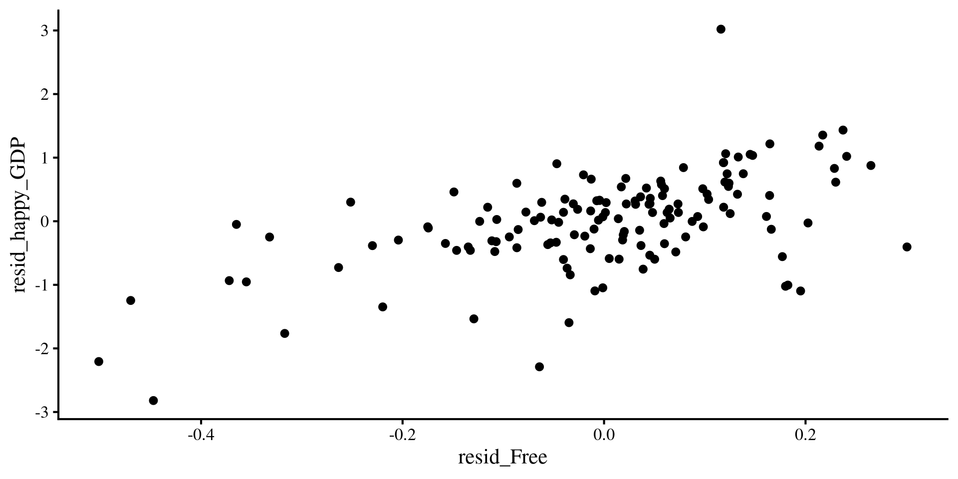

The slopes that you get when you include both predictors are the slopes for the lines of best fit these 2 plots.

The Quick way: avPlots() function from car

car::avPlots(reg_full)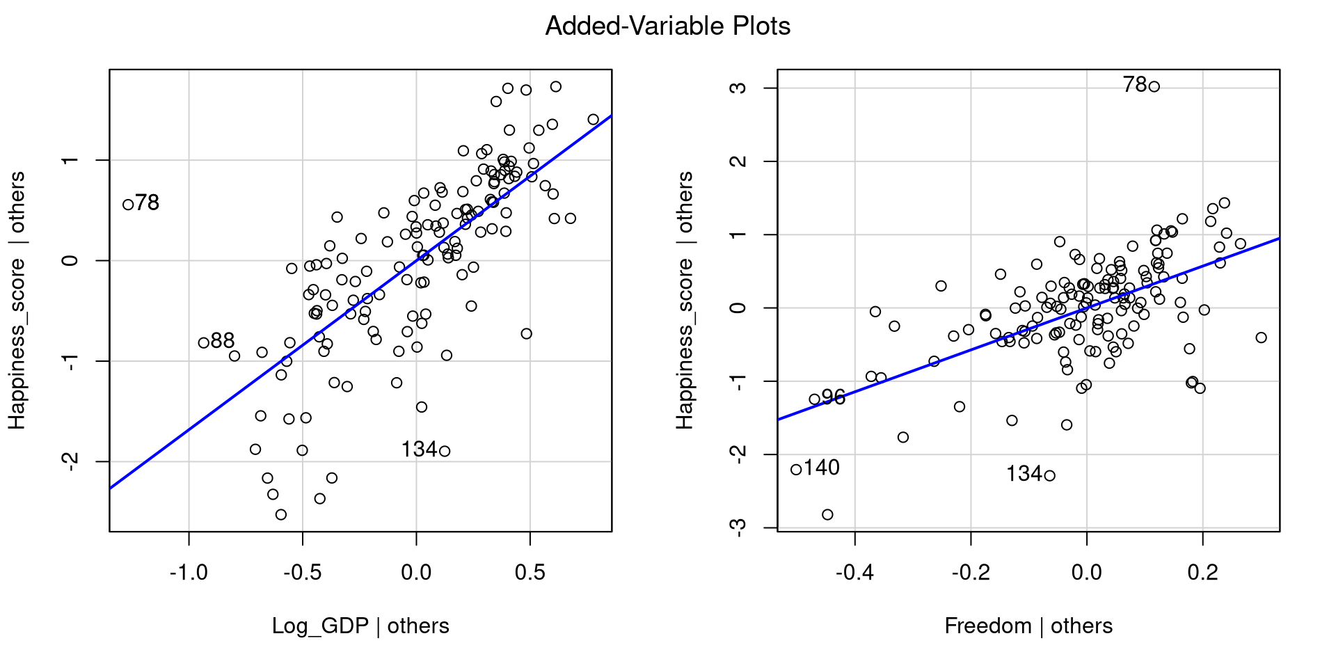

To get added variable plots in practice you would use the avPlot() function.

When you have more than 2 predictors, it is not possible to build a visualization of all variables at once like a 3D plot. Added variable plots can help you visualize regression results no matter the number of predictors!

Another Look at the 3D plane

You can see that the avPlots() function identifies 4 point per plot: 2 points with the highest residuals, and 2 points with the highest leverage

Try tilting the plane such that it resembles the added variable plots on the previous slide. If you hover over the dots in the 3D plot, you should see what point you are looking at (“row #”). Use the points on the added variable plots as a reference.

library(FabioFun)

nice_3D_plot(y = reg_vars$Happiness_score,
             x1 = reg_vars$Log_GDP,
             x2 = reg_vars$Freedom,
             axis_names = c("Happiness", 
                            "GDP", 
                            "Freedom"),
             reg_plane = TRUE)

Bootstrapping

Bootstrapping (Efron, 1992) is a really smart idea to calculate confidence intervals while avoid doing math! You probably have seen some complicated equations that need to be derived to calculate confidence intervals for statistics (e.g., see here for the 95% CI of \(R^2\)).

Turns out that even more complex math goes behind deriving the complicated equations 😱 Usually, that involves figuring out what is the theoretical sampling distribution of a certain statistic for an infinite number of experiments.

Instead bootstrapping says:

“By Hand” Example of Bootstrapping

As always, we can do things ourselves to get a better understanding of the process.

# empty element to save R^2 to
r_squared <- c()

set.seed(34677)

for(i in 1:2000){

# sample from data 
sample <- sample(1:nrow(reg_vars), 
                 replace = TRUE)  

dat_boot <- reg_vars[sample,]

# Run regression
reg_boot <- lm(Happiness_score ~ Log_GDP + Freedom, 
               dat_boot)  

# Save R^2
r_squared[i] <- summary(reg_boot)$r.squared
}

There is a lot of value in understanding how the code above works, but the main point is that we are running the same regression 2000 times with a different sample from our data, and then saving the \(R^2\) that we get every time.

The \(R^2\) from our regression with both variables was

summary(reg_full)$r.squared

[1] 0.7186638

If we look out the distribution of the all the 2000 \(R^2\) we get

# need to run bootstrap code on the left first
hist(r_squared)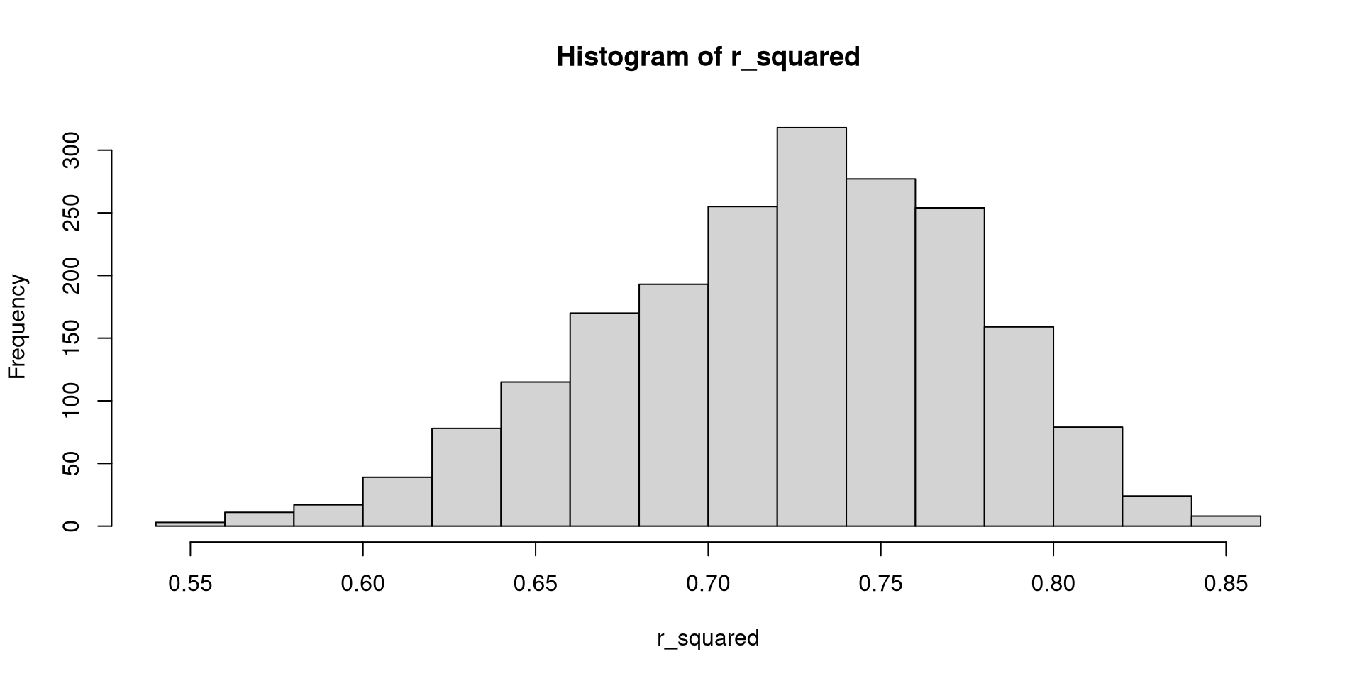

quantile(r_squared, c(.025, .5, .975))

     2.5%       50%     97.5% 
0.6131015 0.7291690 0.8139789 

The Quick way: Boot() function from car

Once again, the car package comes to the rescue

set.seed(875)
boot_model <- car::Boot(reg_full, R = 2000)

confint(boot_model, type = "perc")

Bootstrap percent confidence intervals

                2.5 %   97.5 %
(Intercept) 0.8712328 1.993144
Log_GDP     1.2646729 2.094521
Freedom     1.8735919 3.724216

The confidence interval for \(R^2\) is a bit annoying to get from car, so here we just have the CIs for intercept and slopes

These are our normal confidence intervals from the regression:

confint(reg_full)

                2.5 %   97.5 %
(Intercept) 0.9769482 1.897419
Log_GDP     1.4083851 1.955721
Freedom     2.1432532 3.575151

Bootstrapping becomes more and more accurate as sample size increases. Here it may not be as accurate because we only have 140 observations, although it seems to do alright.

Visualizing Bootstrap Results

You can also visualize the distribution of the bootstrapped samples for the regression slopes.

NOTE: You need to provide the names of the regression slopes as shown in the summary() output through the parm= argument

hist(boot_model, 
     parm = "Log_GDP")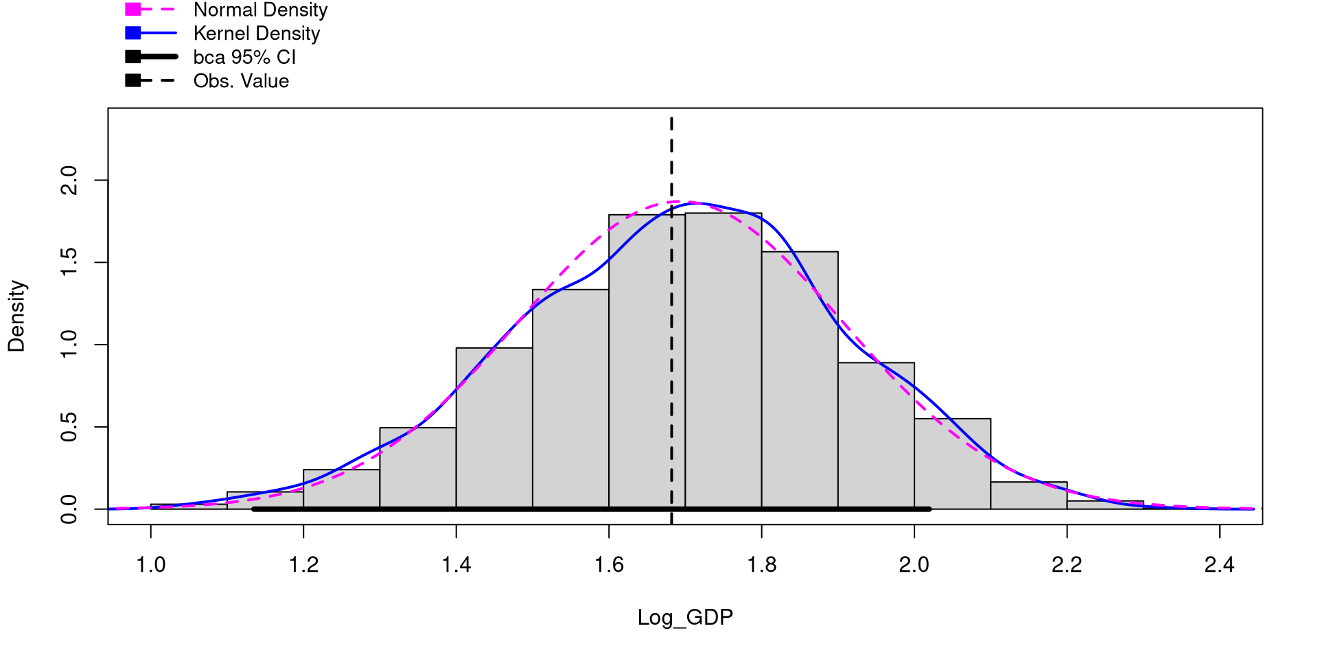

hist(boot_model, 
     parm = "Freedom")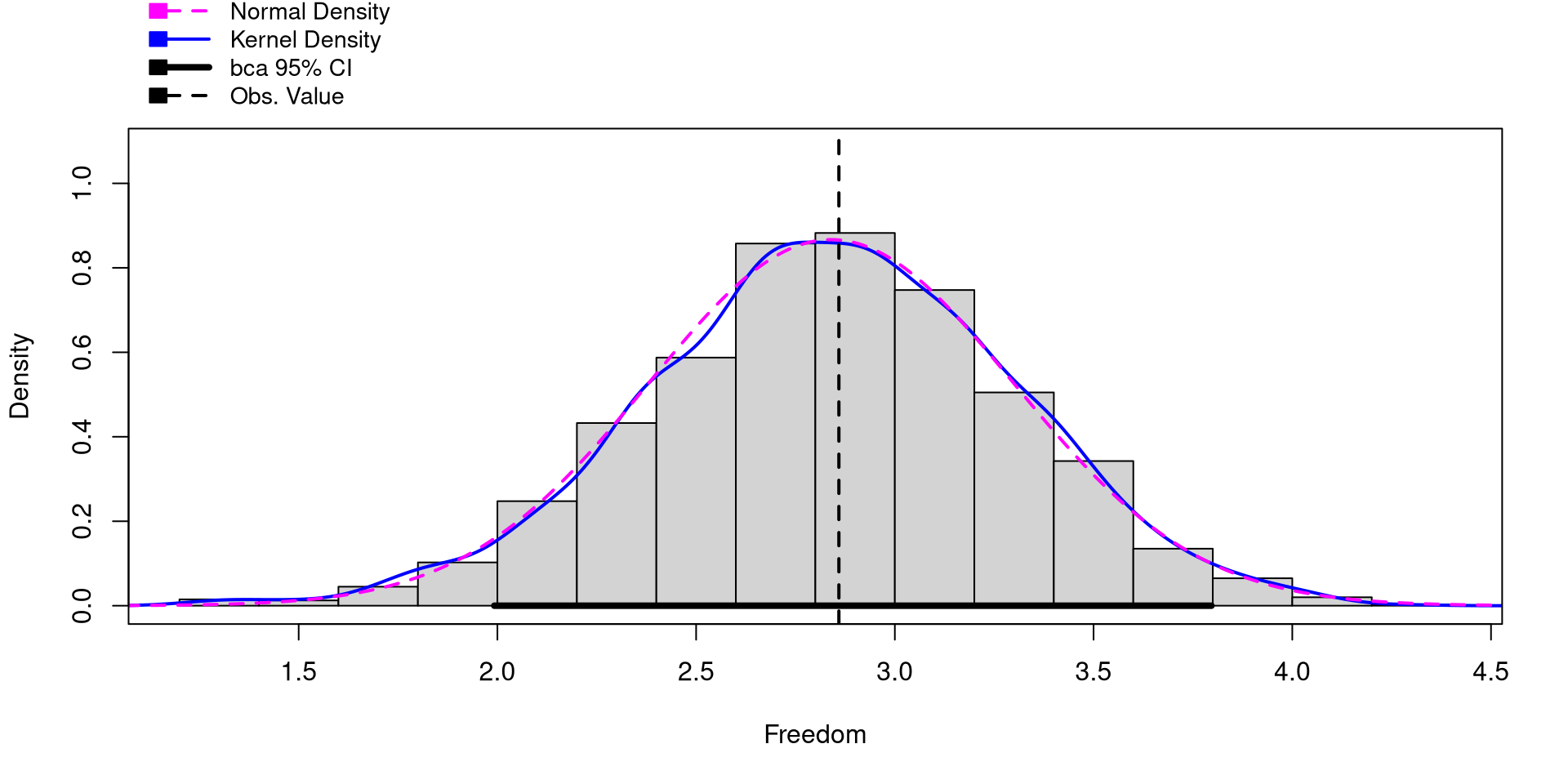

Notice that the bootstrap samples are very normally distributed. This is almost always the case for regression slopes. In contrast, statistics like \(R^2\) will not be normally distributed as we saw 2 slides ago.

References

Efron, B. (1992). Bootstrap Methods: Another Look at the Jackknife. In S. Kotz & N. L. Johnson (Eds.), Breakthroughs in Statistics: Methodology and Distribution (pp. 569–593). Springer. https://doi.org/10.1007/978-1-4612-4380-9_41

Fox, J., Weisberg, S., Price, B., Adler, D., Bates, D., Baud-Bovy, G., Bolker, B., Ellison, S., Firth, D., Friendly, M., Gorjanc, G., Graves, S., Heiberger, R., Krivitsky, P., Laboissiere, R., Maechler, M., Monette, G., Murdoch, D., Nilsson, H., … R-Core. (2024). Car: Companion to Applied Regression (Version 3.1-3) [Computer software]. https://cran.r-project.org/web/packages/car/index.html

Wickham, H., & RStudio. (2023). Tidyverse: Easily Install and Load the ’Tidyverse’ (Version 2.0.0) [Computer software]. https://cran.r-project.org/web/packages/tidyverse/index.html