Lab 4: Introduction To Two-Predictor Regression
PSYC 7804 - Regression with Lab
Helpful Visualization
The ggpairs() function from the GGally package creates a visualizations that provides a lot of information in one go!
ggpairs(reg_vars)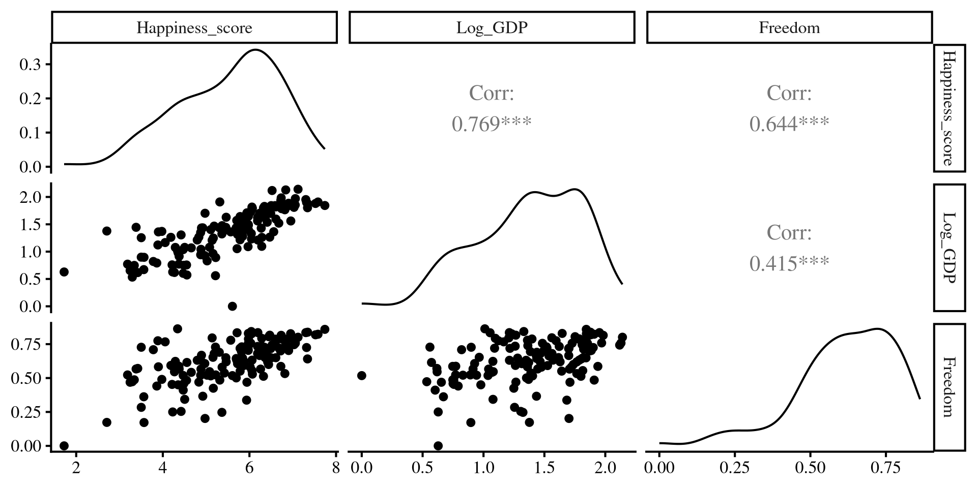
- Upper triangle: correlations among variables
- Long diagonal: distribution of variables
- Lower diagonal: scatterplots among variables
Individual Regression plots
These are the equivalent plots to the individual regressions:
Plot Code
  ggplot(reg_vars,
 aes(x = Log_GDP, y = Happiness_score)) +
 geom_point() +
    geom_smooth(method = "lm",
                formula = "y~x",
                se = FALSE)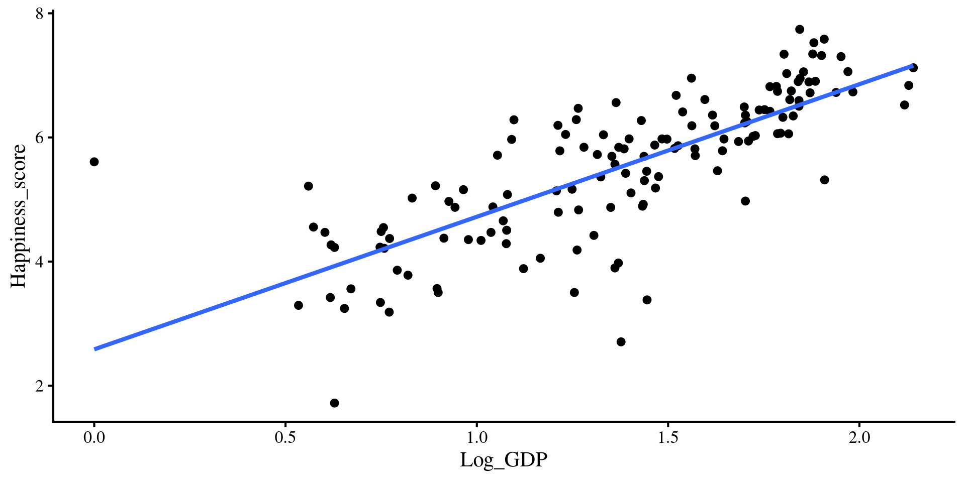
Plot Code
  ggplot(reg_vars,
 aes(x = Freedom, y = Happiness_score)) +
 geom_point() +
    geom_smooth(method = "lm",
                formula = "y~x",
                se = FALSE)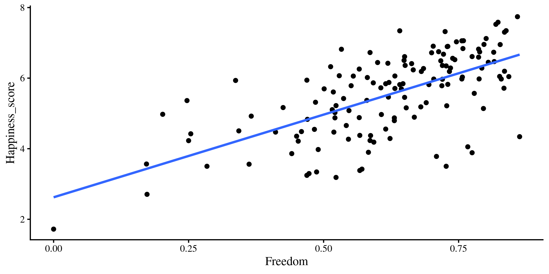
Adding Slopes from multiple regression?
Let’s add the regression lines estimated from the regression with both predictors…
Plot Code
  ggplot(reg_vars,
 aes(x = Log_GDP, y = Happiness_score)) +
 geom_point() +
    geom_smooth(method = "lm",
                formula = "y~x",
                se = FALSE) +
    geom_abline(intercept = coef(reg_full)[1],
                slope = coef(reg_full)[2])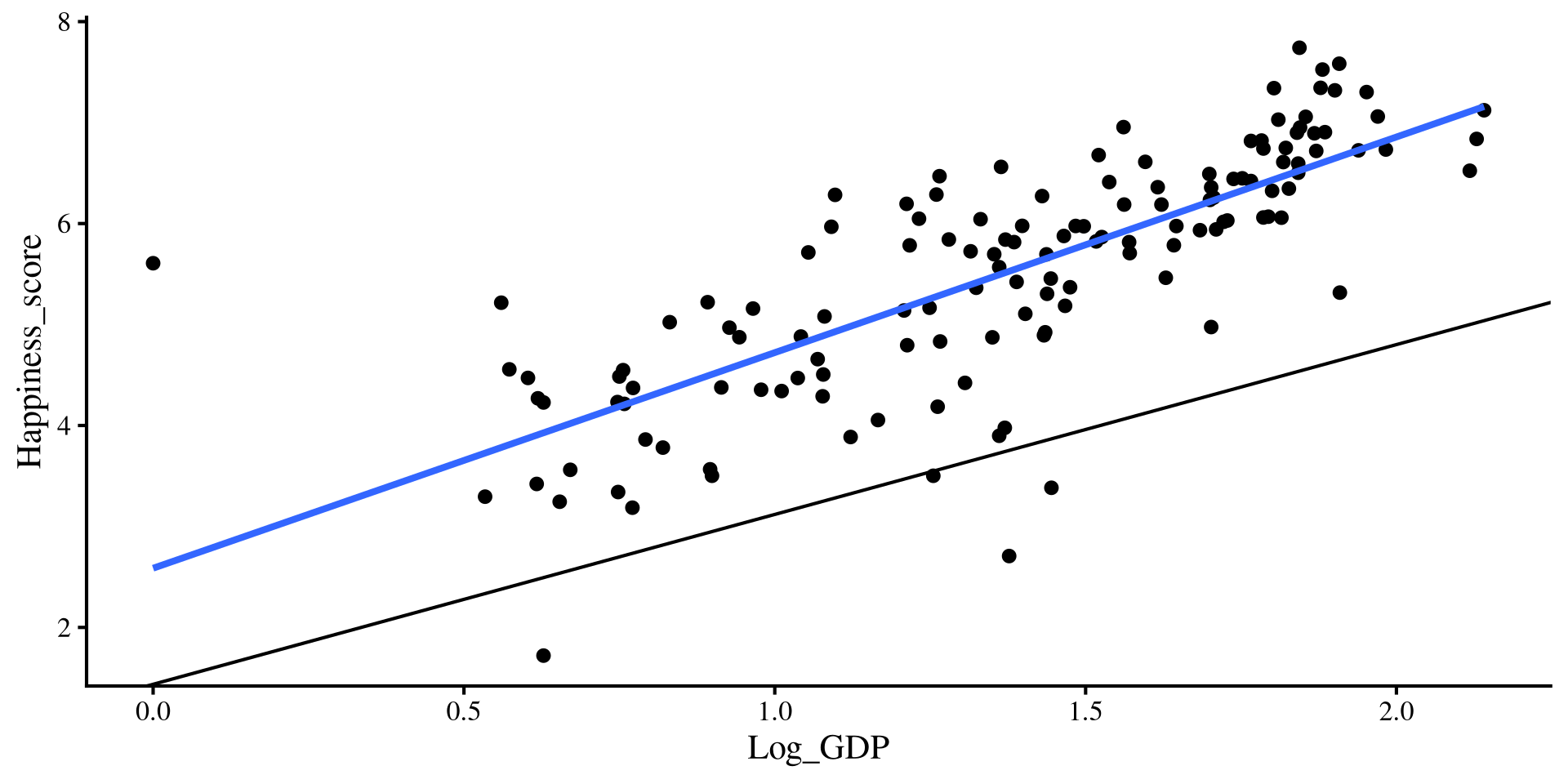
Plot Code
  ggplot(reg_vars,
 aes(x = Freedom, y = Happiness_score)) +
 geom_point() +
    geom_smooth(method = "lm",
                formula = "y~x",
                se = FALSE) +
    geom_abline(intercept = coef(reg_full)[1],
                slope = coef(reg_full)[3])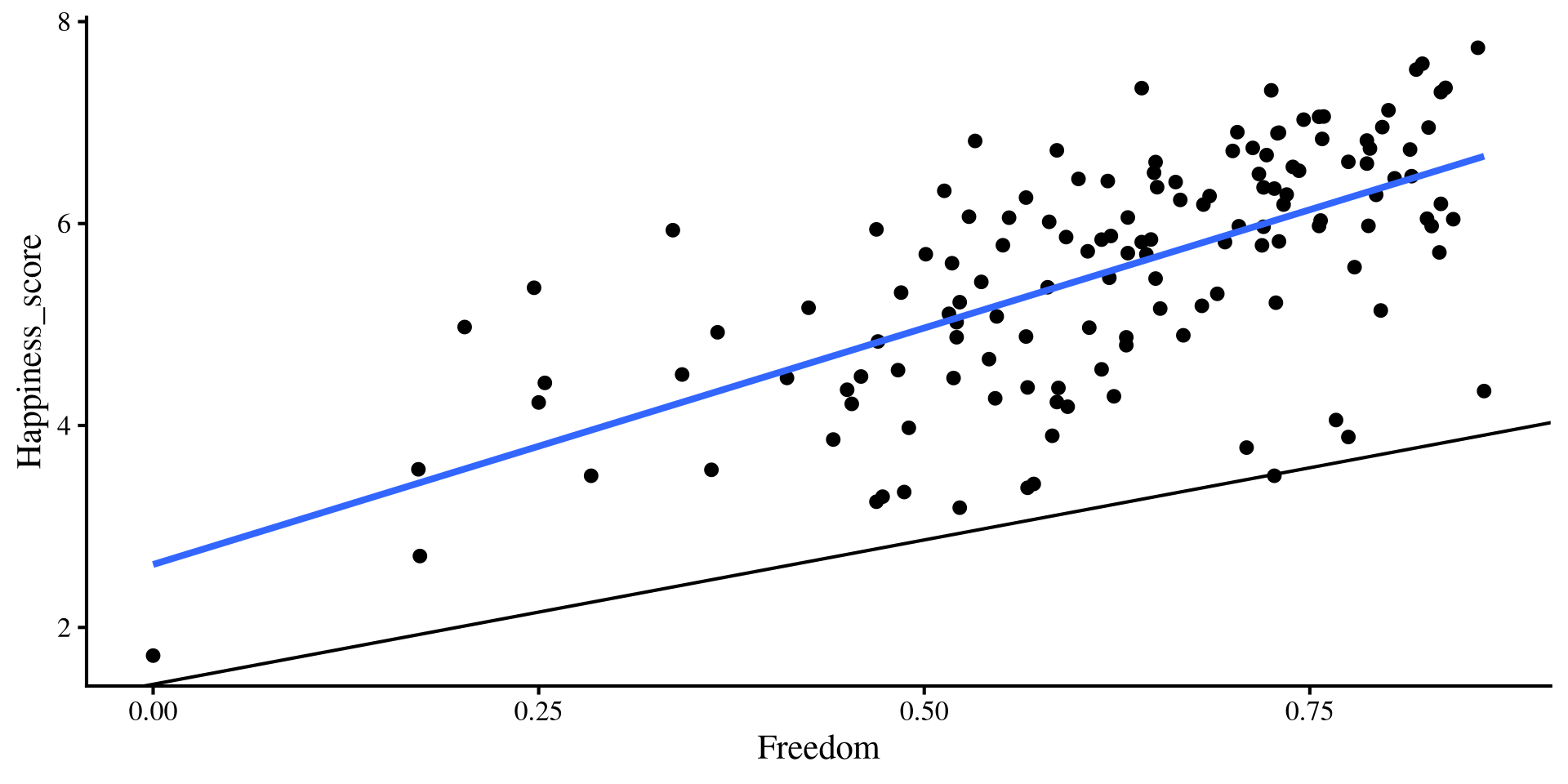
Hold up, the lines from the multiple regression results seem way off !?
💡 Maybe we need a change of perspective!
Back to our friend R 2
You can think of variance as how unpredictable something is. Higher variance means more unpredictability. At the same time, no variance means perfect predictability!
For example, if you generate data for a variable that has 0 variance, you always get the mean
rnorm(n = 5,
      mean = 2,
      sd = 0)
[1] 2 2 2 2 2Here, if we predict 2 we are always right, because the variable has no variance and is perfectly predictable.
Let’s return to our 1D scatterplot, and let’s visualize the variance of the Happiness_score
Code
ggplot(reg_vars,
       aes(x = Happiness_score, y = 0)) +
       geom_point(shape = 1,
                  size=6.5) +
      annotate("text", x = 4.7, y = .02,
             label = "Variance of Happiness_score") +
xlim(1.5, 8.2) +
    ylim(-.1, .03) +
  theme(axis.title.y=element_blank(),
        axis.text.y=element_blank(),
        axis.ticks.y=element_blank(),
        axis.line.y =  element_blank())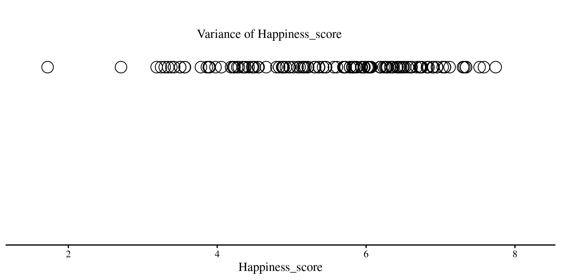
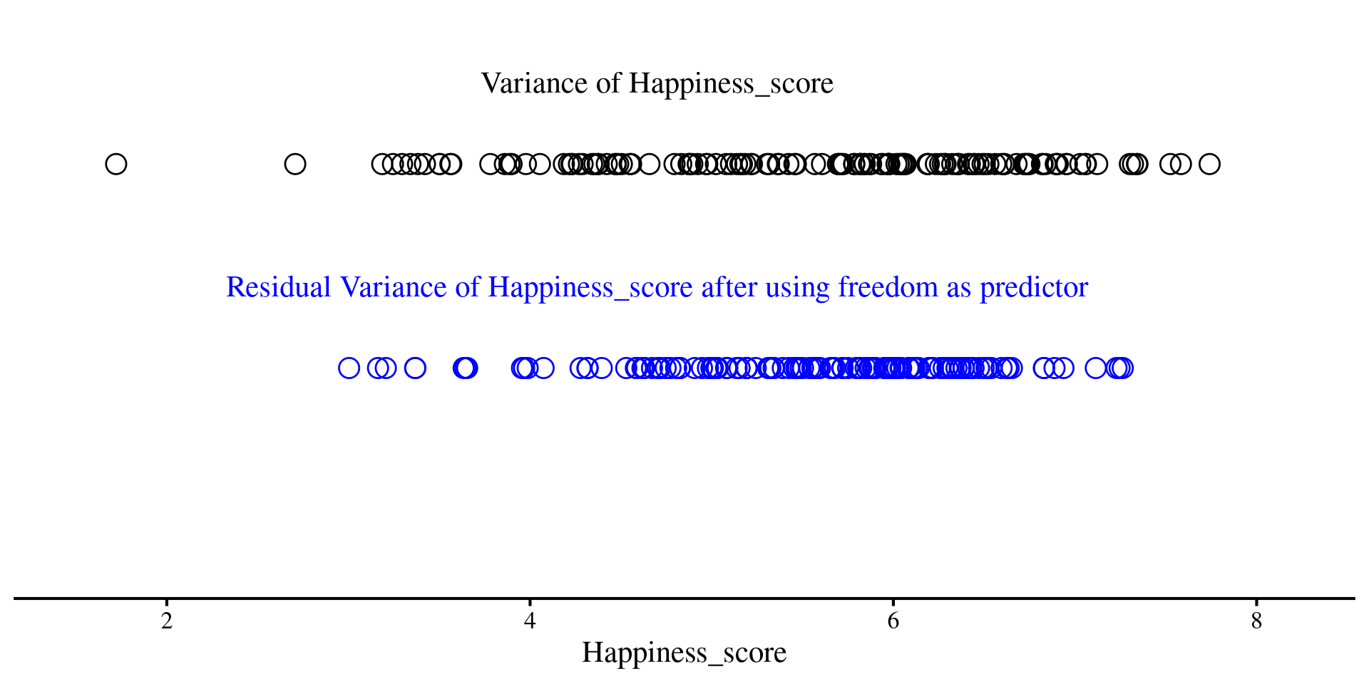
Variance of Residuals after regression
Although this may not sound very intuitive, you should think of residuals as a new version of your \(Y\) variable, but with some unpredictability taken out thanks to our regression line. Less unpredictability means lower variance
On the right, we have the residuals of Happiness_score after using freedom as predictor
Code
ggplot(reg_vars,
       aes(x = Happiness_score, y = 0)) +
       geom_point(shape = 1,
                  size=4.5) +
      annotate("text", x = 4.7, y = .02,
             label = "Variance of Happiness_score") +
  geom_point(aes(x = residuals(reg_free) +
                       # add mean to have residuals on same scale as
                       # previous graph (variance remains the same)
                         mean(reg_vars$Happiness_score),
                     y = -.05),
             shape = 1,
             size = 4.5, color = "blue") +
        annotate("text", x = 4.7, y = -0.03,
             label = "Residual Variance of Happiness_score after using freedom as predictor", color = "blue") +
xlim(1.5, 8.2) +
    ylim(-.1, .03) +
  theme(axis.title.y=element_blank(),
        axis.text.y=element_blank(),
        axis.ticks.y=element_blank(),
        axis.line.y =  element_blank())
Much less spread out, right?
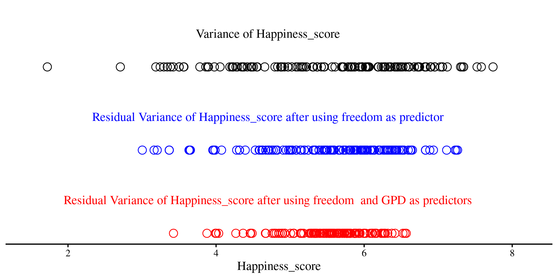
Variance of Residuals after Regression
Although this may not sound very intuitive, you should think of residuals as a new version of your \(Y\) variable, but with some unpredictability taken out thanks to our regression line. Less unpredictability means lower variance
Now, after we add both freedom and GDP as predictors, we see that the dots are even less spread out
Code
ggplot(reg_vars,
       aes(x = Happiness_score, y = 0)) +
       geom_point(shape = 1,
                  size=4.5)+
      annotate("text", x = 4.7, y = .02,
             label = "Variance of Happiness_score") +
  geom_point(aes(x = residuals(reg_free) +
                       # add mean to have residuals on same scale as
                       # original variable (variance remains the same)
                         mean(reg_vars$Happiness_score),
                     y = -.05),
             shape = 1,
             size = 4.5, color = "blue")  +
        annotate("text", x = 4.7, y = -0.03,
             label = "Residual Variance of Happiness_score after using freedom as predictor", color = "blue") +
  geom_point(aes(x = residuals(reg_full) +
                       # add mean to have residuals on same scale as
                       # original variable (variance remains the same)
                         mean(reg_vars$Happiness_score),
                     y = -.1),
             shape = 1,
             size = 4.5, color = "red") +
  annotate("text", x = 4.7, y = -0.08,
             label = "Residual Variance of Happiness_score after using freedom  and GPD as predictors", color = "red") +
xlim(1.5, 8.2) +
    ylim(-.1, .03) +
  theme(axis.title.y=element_blank(),
        axis.text.y=element_blank(),
        axis.ticks.y=element_blank(),
        axis.line.y =  element_blank())
The red dots are even less spread out than the blue ones!
P-value from the \(F\)-distribution
We want to calculate how likely it is to get our \(F\)-value from an \(F\)-distribution with \(\mathrm{df}_1 = k = 2\), and \(\mathrm{df}_2 = \mathrm{df_{residual}} = 137\).
If we look at our full regression, our \(F\)-value was \(\frac{\mathrm{df_{residual}}\times R^2}{k(1 - R^2)} = \frac{137\times .63}{2(1 - .63)} \approx 175\)
You can see that \(175\) is way off to the right. The probability of getting \(175\) or more from this distribution is the \(p\)-value:
# the probability for the F-distribution
pf(175, df1 = 2, df2 = 137, lower.tail = FALSE)
[1] 1.86048e-38
So, extremely unlikely (\(p = 1.86\times10^{-38}\)) to see \(F = 175\) from the distribution on the right if \(R^2 = 0\). We reject \(H_0\).
Plot Code
ggplot() +
  geom_function(
    fun = df,
    args = list(df1 = 2, df2 = 137),
    col = "blue") +
  labs(x = "All Possible F-values if R\U00B2 = 0",
       y = "Density") +
  xlim(0, 10)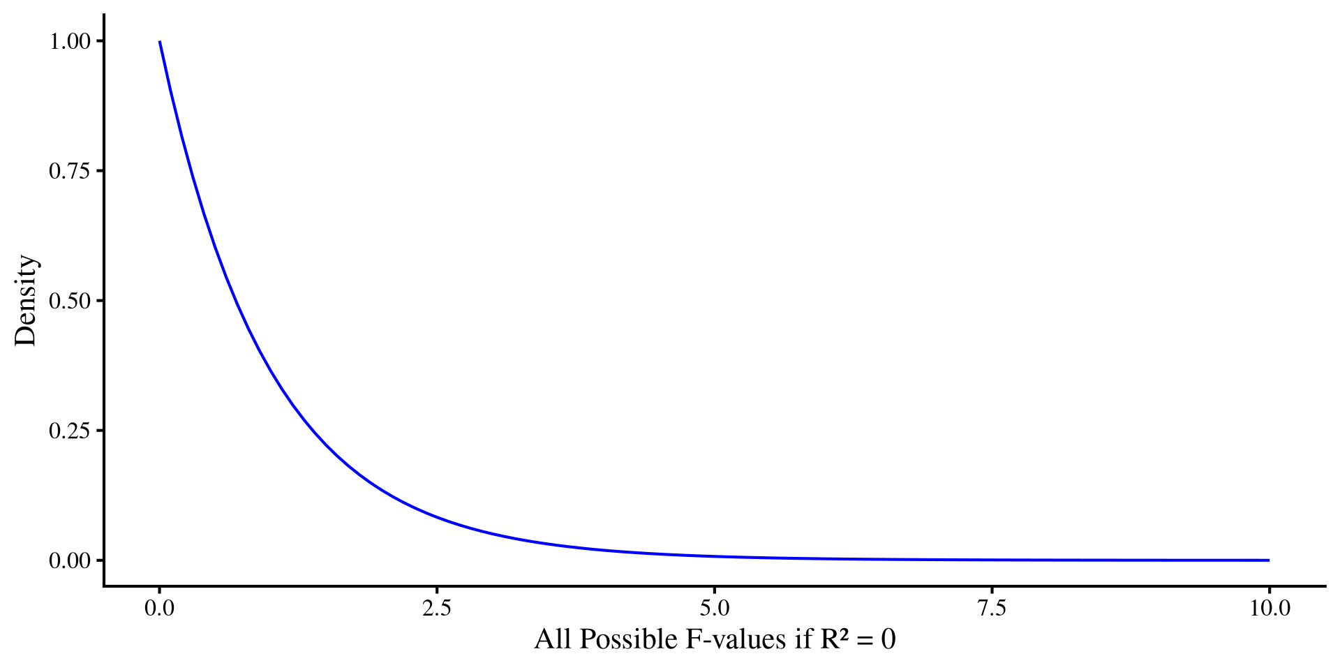
Simulating Experiments where \(H_0\) is true
The idea of sampling distributions can be a bit abstract. To convince myself that smart math people are not lying to me, I sometime simulate things; simulating a large (not quite infinite) number of experiments if pretty straightforward in R!
sample_size <- 300

# object where we save F-statistic
F_statistics <- c()

for(i in 1:2000){

X <- rnorm(sample_size, mean = 0, sd = 1)
# the regression coefficient of X is exactly 0
Y <- rnorm(sample_size, mean = 0*X, sd = 1)

reg_YX <- lm(Y ~ X)

# store F-statistic at every iteration
F_statistics[i] <-  as.numeric(summary(reg_YX)$fstatistic[1])
}

ggplot() +
  geom_density(aes(x = F_statistics)) +
      scale_y_continuous(expand = c(0, 0))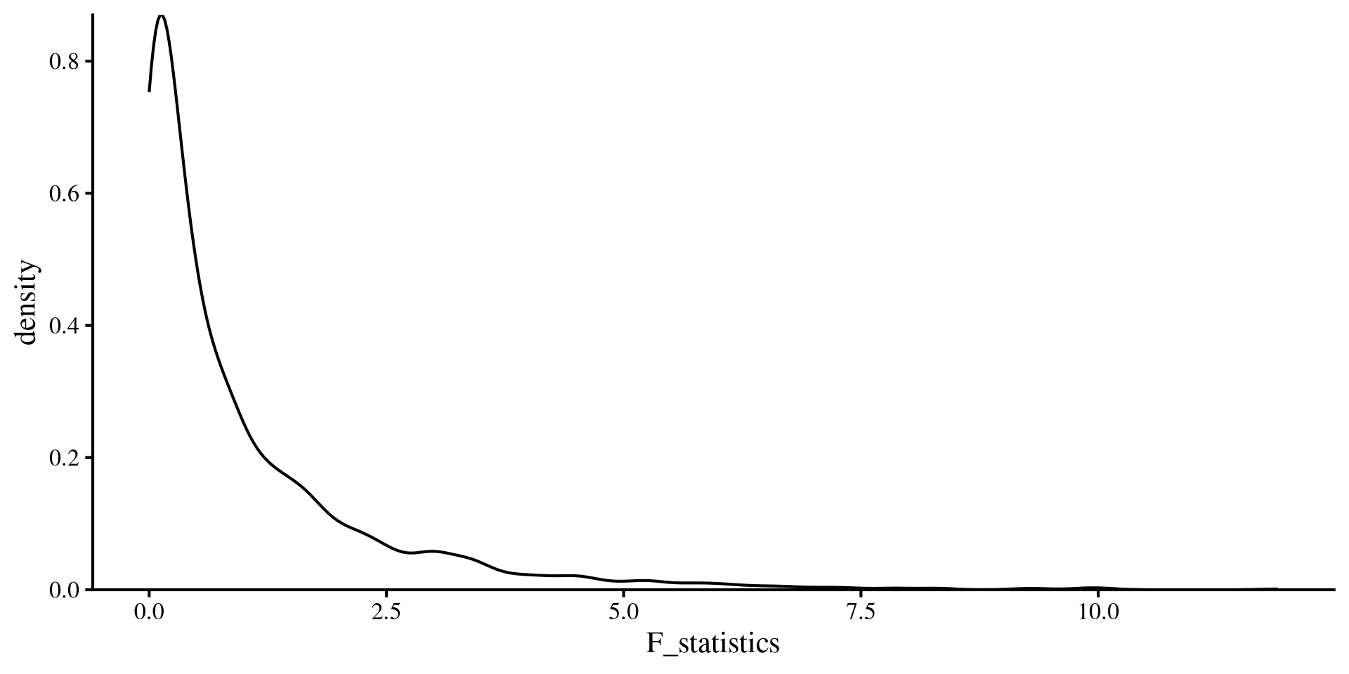
On the left, there is code that simulates 2000 “experiments” with one predictor and \(N = 300\) where \(R^2 = 0\). If we save the \(F\)-values from each experiment and plot them, you will see that the plot matches an \(F\)-distribution with \(\mathrm{df}_1 = 1\) and \(\mathrm{df}_2 = 298\). Check with the plot on the previous slide! (make sure the range of the x-axis match)