Lab 13: Missing Data
PSYC 7804 - Regression with Lab
Spring 2025
Today’s Packages and Data 🤗
The naniar package (Tierney et al., 2024) provides tools to summarize, visualize, and explore missingness in your data. Check out the packege’s website to find out more.
The missMethods package (Rockel, 2022) includes functions to create, handle, and evaluate missing data. In this lab I just use some functions from this package to simulate missing data.
This data is taken from this website, which I talk about on the next slide.
This is some fabricated data about 630 employees who filled out a work satisfaction survey at a company. The meaning of the individual variables is not super important.
We will also use lavaan to run regressions, so I load this function to have clearer summaries later:
For all your missing data needs
This lab is a very quick overview of some methods of dealing with missing data. More often than not, your missing data woes will be trickier than what I go over here.
As far as missing data resources go, I would say that Applied Missing Data Analysis (Enders, 2022) is the best resource at the time of making these slides.
I think the book is very approachable, and explains many of the concepts very clearly!
Additionally, there is a website that complements the book very nicely. You can also find the code for the examples from each chapter on the website.

Software Behavior With Missing Data?
We have 630 observations, but let’s say that the when we collected our data, the first 300 observations in our data are missing on the climate variable, which I am going to define as climate_miss.
Even though our sample size is 630, and values are missing only for climate_miss, the lm() function discarded all of those observations. We lost 300 observations for having missing values on a single predictor 😱
This is called listwise deletion, and most software will do this by default. More practically you will lose a large portion of your sample without realizing it!
The more important issues is that, in many instances, listwise deletion will also lead to biased results. We will return to this in a couple of slides.
Why is My Data Missing?
There may be many reasons why you end up with missing data. In general, there are 3 missing data mechanisms that can describe the way in which data is missing:
Missing completely at random (MCAR)
Missing data is said to be MCAR if the missing values in your data happen completely at random, meaning that there is no discernible pattern in the missingness.
Missing at Random (MAR)
Missing data is said to be MAR if the missing values in your can be predicted by your observed variables, meaning that some of your measured variables explain why data may be missing.
Missing not at random (MNAR)
Missing data is said to be MAR if the missing values are due to some variable that is not observed. This is the worst case of missing data because something that you don’t know about is causing your data to disappear.
I am using the terminology from Enders (2022), you may see different names for these 3 mechanisms.
Regardless, these processes are important because methods that deal with missing data make the assumption that one of these three mechanisms are at play.
Bias
What is so bad about missing data? Well, as foreshadowed the main problem is that if the missingness is MAR or MNAR, you will get biased results if you don’t account for the missingness process appropriately. Bias has a very specific meaning in statistics. For example:
One of the tenets of statistics is that if you somehow managed to measure the entire population on something, you would be able to calculate the true value of a statistics (e.g., correlation, regression slope, mean,…).
Let’s say that we managed to measure every person in the world and we observed that the correlation between income and happiness is \(r = .2\). However, in my sample of 200 US citizens I find a correlation of \(\hat{r} = .4\).
In this case, \(\mathrm{bias} = \hat{r} - r = .4 - .2 = .2\).
Thus, bias is the expected difference between the true value of a statistic and the observed value. All of statistical theory rests on the assumption that our sample is representative of the population, and can therefore produce unbiased estimates of the true population statistic we want to know.
Example of Bias: The Population
As practical example, I’ll simulate some hypothetical data where students are admitted to grad school regardless of their GRE score. For this made up data, the correlation between Graduate_GPA and GRE_Score is:
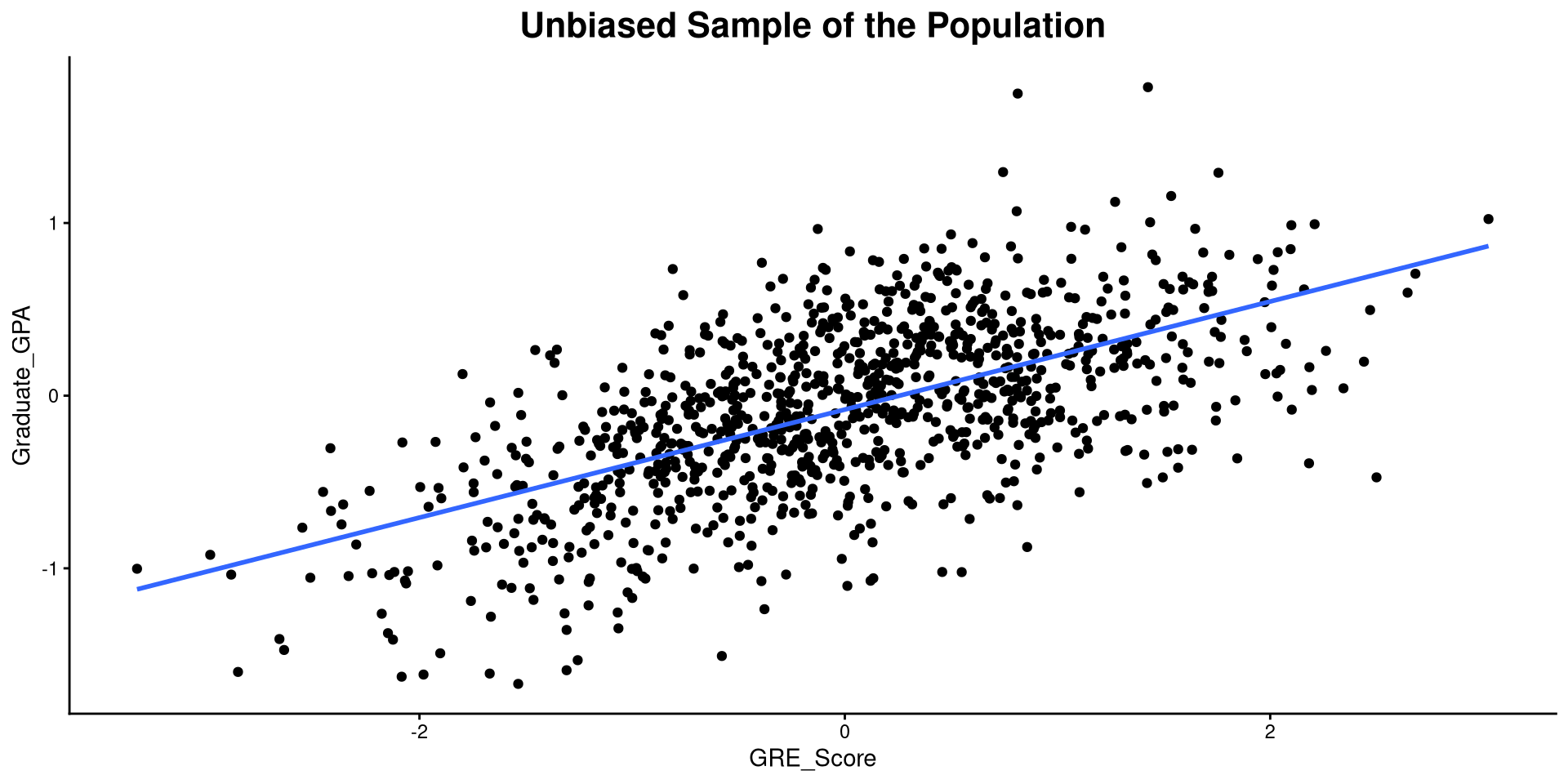
In reality, students with low GRE scores are not usually admitted to graduate programs, so their GPA is not observed 🧐 Let’s see what happens to our correlation in that case…
Example of Bias: Biased Sample
If only students who have a GRE score at the mean or above are admitted to graduate programs, then the correlation Graduate_GPA and GRE_Score becomes:
Compared to the previous plot, we only observe values with GRE_Score \(> 0\), which causes us to think that the correlation between Graduate_GPA and GRE_Score is lower than it actually is in reality 🤔
This a case of bias due to restriction of range.
Plot code
ggplot(bias_dat[bias_dat$GRE_Score > 0,] , aes(x = GRE_Score, y = Graduate_GPA))+
  geom_point() +
  geom_smooth(method = "lm", se = FALSE) +
  theme_classic() +
         labs(title = "Biased Sample of the Population",
            y= "GPA",
            x = "Test Score") +
   theme(plot.title = element_text(hjust = 0.5, face = "bold", size = 16))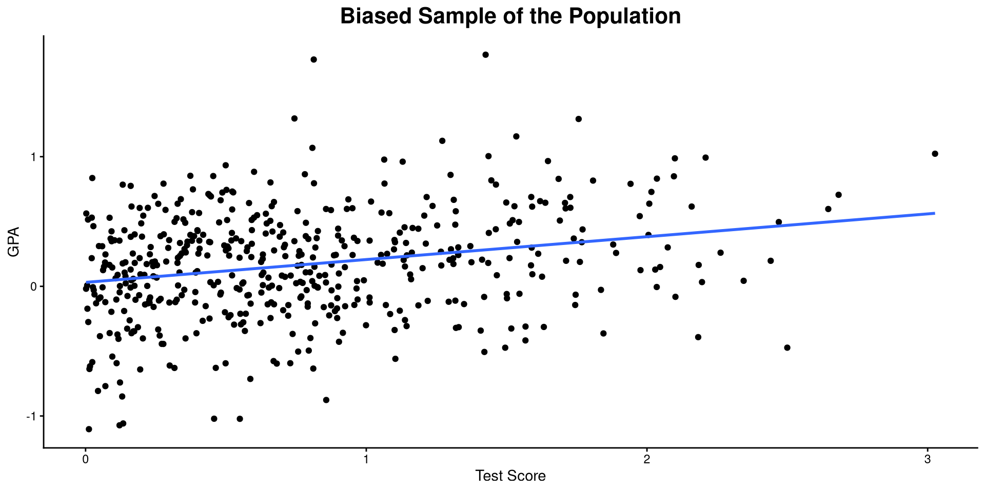
Missing Data and Bias
In the previous example, we saw that the true correlation between Graduate_GPA and GRE_Score was \(r = .61\), but in our sample we found that \(\hat{r} = .25\). This is some pretty serious bias, which will cause us to make some very different conclusions about our hypotheses.
What does this have to do with missing data? The example from before is actually a missing data problem, where missingness in Graduate_GPA is caused by GRE_Score (MAR process). Going back to our missing data processes, two of them will result in biased results if cases are deleted like we just did.
Missing completely at random (MCAR)
Will not produce bias if cases are deleted
Missing at Random (MAR)
Will produce bias if cases are deleted
Missing not at random (MNAR)
Will produce bias if cases are deleted
By default, most software delete cases if any of them are missing on a single variable (e.g., lm() will delete rows if they are missing on a single predictor/outcome), which causes bias unless missingness is completely random (MCAR). Of course, this is not a big problem if you only delete few cases.
Can I know How My Data Went Missing?
Depending on how our data went missing, we have to use different methods to prevent bias. However, how do we find out whether our missing data is MCAR, MAR, or MNAR? Unfortunately, The only thing we can find out is whether our missingness is MCAR or not 🤷
- Testing MAR would require you to know for sure that there is no unobserved variable that predicts missingness beyond the variables in your data (impossible 🤷)
- Testing MNAR would require you to know for sure that there is an unobserved variable that predicts missingness (impossible 🤷)
To test MAR and MNAR you would have to know about a variable that you don’t know about (a statement worthy of a philosophy PhD dissertation).
Ok, but how do we know that methods of handling missing data work/do not work or produce more or less bias? There is no empirical way to test this because either you the full data or you do not (you do not have both to compare). The only way is to have a complete dataset and then simulate different missingness mechanisms, which is what we are going to do for the rest of this class.
Little’s MCAR test
To test that missingness in your data is MCAR you can use the mcar_test() function from the naniar package, which runs Little’s MCAR test (Little, 1988). If the data is indeed MCAR, the result will not be significant.
delete_MCAR() function and then use mcar_test()
worksat) are less likely to report the other variables when asked:
Generate MAR
set.seed(467)
# Probabilities of missingness based on `worksat`
mis_prob <- 1 - plogis(dat$worksat, location = mean(dat$worksat), scale = sd(dat$worksat))
dat_miss_MAR <- dat

# MAR process for other variables
for(i in 1:4){
  dat_miss_MAR[,colnames(dat)[-3][i]] <- ifelse(rbinom(nrow(dat), 1, mis_prob) == "1", NA, dat[,colnames(dat)[-3][i]])
}Non-Significant Little’s Test?
When Little’s test is not significant, you are in the clear! Even if you delete observations with missing data, your results will not be biased. Don’t trust me? Let’s run a quick simulation!
We want to see how empower, lmx, climate, and cohesion predict worksat. First we run the regression with the complete data to use the result as a comparison.
(Intercept)     empower         lmx     climate    cohesion
      0.532       0.021       0.161       0.073      -0.033
Here are the intercept and slopes for our regression when we have the full data.
Now that we know what the results should look like we can simulate missingness mechanisms, run the regression again, and check how far we are from the values on the left.
We are treating the values on the left as the population values.
Remember that the lm() function will delete any rows that have a missing value on any of the variables. So, we should expect bias when missingness is MAR, but not when missingness is MCAR.
MCAR VS MAR with lm()
I am going to simulate both MCAR and MAR many times, run regressions with lm() each time, and then look at the average values of the intercepts and slopes:
(Intercept)     empower         lmx     climate    cohesion
      0.532       0.021       0.159       0.074      -0.032
MCAR: Almost the same as the previous slide!
MAR Sim Code
set.seed(4627)


MAR_list <- list()
mis_prob <- 1 - plogis(dat$worksat, location = mean(dat$worksat), scale = sd(dat$worksat))

for(i in 1:2000){

dat_miss_MAR <- dat

# MAR process for other variables
for(j in 1:4){
  dat_miss_MAR[,colnames(dat)[-3][j]] <- ifelse(rbinom(nrow(dat), 1, mis_prob) == "1", NA, dat[,colnames(dat)[-3][j]])
}

MAR_list[[i]] <-  coef(lm(worksat ~ empower + lmx + climate + cohesion, dat_miss_MAR))

}

MAR_res <- bind_rows(MAR_list)MAR: Definitely much more biased!!
So, if you have a bunch of observations disappearing due to missing cases, check that the data is MCAR before running regressions on it. You may be getting biased results like the one of the right. Some notes on the code:
Are My Results Truly Unbiased?
Probably not. Although I showed that when missingness is MCAR, listwise deletion will produce unbiased results, that is only true on average (colMeans()) over many replications. If you look inside the MCAR_res object you will see the results for all the replications, and some of them will indeed be biased. The only assurance that statistics can give you is that on average you will be fine, not that you will always be fine.
Significant Little’s Test?
When Little’s test is significant, you need to be careful! You know for sure that your missing data is not MCAR. So what next?
❌ You probably should not just use the lm() function, which does listwise deletion when rows have missing cases, and will likely produce biased results as shown on the previous slide.
✅ Instead, we should use full information maximum likelihood (FIML) to estimate our regression. lavaan can run FIML for missing data. There are 2 big advantages that FIML provides:
-
Your results will be less biased if missing data is MAR. If the data is MCAR, FIML will work just as well as
lm(). - You will not lose any observations and you will retain your full sample! This helps with power (if you are into that kind of stuff), but also makes results more reliable.
Note that FIML “works” only if your missing data is either MCAR or MAR; if data is MNAR, meaning that you have no measured variable that is related to missingness, then FIML will not be of much help and you’ll need some more sophisticated stats.
FIML with lavaan
Running FIML in lavaan just involves adding a few extra arguments to the sem() function!
# parameterestimates(fit_miss)[16, 4] gets the intercept for this specific model (do not copy and paste this line and expect it to print the intercept for other models, it will not work; you need to look for it through the lavaan summary yourself usually)
round(c(parameterestimates(fit_miss)[16, 4],
        lav_summary(fit_miss)[,4]), 3)
[1] 0.384 0.011 0.180 0.068 0.043Close to the original values below!
Here, dat_miss_MAR is the last dataset generated from the MAR simulation on from two slide ago. Some notes on the code:
-
meanstructure = TRUE: askslavaanto also estimate the intercepts, which it does not do by default. -
fixed.x = FALSE: without going in too much detail, this is necessary forlavaanto be able to use FIML. -
missing = "fiml": tellslavaanto use FIML to estimate the model, which helps reducing bias if missing data is MAR.
This is an example with just a single dataset, so check out the next slide to see how much better FIML is on average compared to listwise deletion for MAR data.
Comparing lm() and lavaan With MAR data
lm() Sim Code
set.seed(4627)


MAR_list_lm <- list()
mis_prob <- 1 - plogis(dat$worksat, location = mean(dat$worksat), scale = sd(dat$worksat))

for(i in 1:2000){

dat_miss_MAR <- dat


# MAR process for other variables
for(j in 1:4){
  dat_miss_MAR[,colnames(dat)[-3][j]] <- ifelse(rbinom(nrow(dat), 1, mis_prob) == "1", NA, dat[,colnames(dat)[-3][j]])
}

MAR_list_lm[[i]] <-  coef(lm(worksat ~ empower + lmx + climate + cohesion, dat_miss_MAR))

}

MAR_res_lm <- bind_rows(MAR_list_lm)FIML Sim Code
# this will take around 10 minutes to run (could be faster if I parallelized loops)
library(lavaan)

set.seed(4627)

MAR_list_fiml <- list()
mis_prob <- 1 - plogis(dat$worksat, location = mean(dat$worksat), scale = sd(dat$worksat))
lav_mod <- "worksat ~ empower + lmx + climate + cohesion"

for(i in 1:2000){

dat_miss_MAR <- dat

# MAR process for other variables
for(j in 1:4){
  dat_miss_MAR[,colnames(dat)[-3][j]] <- ifelse(rbinom(nrow(dat), 1, mis_prob) == "1", NA, dat[,colnames(dat)[-3][j]])
}


fit_miss <- lavaan::sem(lav_mod, dat_miss_MAR, meanstructure = TRUE, fixed.x = FALSE, missing = "fiml")

MAR_list_fiml[[i]] <-  c(parameterestimates(fit_miss)[16, 4], lav_summary(fit_miss)[,4])

print(paste("iter", i))

}

MAR_res_fiml <- matrix(unlist(MAR_list_fiml), ncol = 5, byrow = TRUE)As you can see, when we simulate MAR missingness, the results produced by lavaan are, on average, closer to the original results. You can especially see the benefits for the intercept and the slope of lmx.
So, when Little’s test is significant and you need as quick solution, FIML is your best bet. On the next slide, I touch upon some other missing data methods/topics that you may want to look into when FIML estimation alone does not cut it.
Further Topics
In no particular order, there are many more topics that require much more time to be covered. All of them are covered in detail in Enders (2022). Some notable ones:
Auxiliary variables
You can think of auxiliary variables as covariates, but they are variables that help you predict missing values and allow FIML (or multiple imputation methods) to get more accurate results. The semTools package (Jorgensen et al., 2025) has a function that lets you add auxiliary variables to lavaan’s models.
Multiple imputation
mice package (Buuren et al., 2024) can do multiple imputation.
MNAR data
Although MNAR is untestable, if your data is not MCAR, and you have no measured variables that explain why data may be missing, then you are in the MNAR territory. Two statistical methods that you need to look into in this case are selection models and pattern mixture models. This document is a good place to start.
References
PSYC 7804 - Lab 13: Missing Data