Lab 14: Repeated Measures
Fabio Setti
PSYC 6802 - Introduction to Psychology Statistics
Today’s Packages and Data 🤗
The ez package (Lawrence, 2016) is a package designed to make ANOVAs analysis in R easier and more intuitive. It has some nice features, but does some things that I don’t personally love.
The lme4 package (Bates et al., 2025) is a popular package for running hierarchical linear modeling (HLM) in R.
The lmerTest package (Kuznetsova et al., 2020) builds upno lme4 and provides addition summary information.
The performance package (Lüdecke et al., 2025) provides a host of function to evaluate the performance and quality of HLM models.
Today we will look at data from (Schmidt & Besner, 2008), where the authors investigate how levels of rewards impacted performance on the Stroop task:
From Wide data to long Data
The data that we have on the previous slide is wide data. Most repeated measures packages prefer by far long data. We can use the pivot_longer() function from the dplyr package to turn wide data into long data:
And now dat_long looks like this:
cols =: here you select the column of the data that you want to “stack”. Note that other columns in the data will automatically be sorted approprtiately as happened with theSubjectcolumn.
names_to =: here you define a new column where the labels for each value will end up.
values_to =: here you define a new column where your numerical values will end up.
There is also a function called pivot_wider() that can turn the data from long into wide.
Repeated-Measures ANOVA with ez
The ezANOVA() function from the ez package is convenient for running repeated measure ANOVA.
As always, it is good practice to turn categorical variables into factor variables:
The ezANOVA() function works slightly differently compared to what we have seen before:
data =the name of your dataset.dv =this is the name of your dependent variable (DV).wid =this is the column that indicates the ID of each participant.within =this is you independent variable (IV). The “within” means that every individual experiences multiple levels of the IV (i.e., the repeated measures part).
A between = argument is also available for running “normal” (between-subject) ANOVAs.
Repeated-Measures ANOVA Results
The results are store in the ANOVA element. We can just print it to look at the results:
The Effect of Contingency is significant, emaning that there are error rates differences in the stroop task depending on the type of reward. ges stands for generalized eta squared and is a measure of effect size; here, it is very small at roughly \(\eta = .01\).
We can also test whether the sphericity assumption has been violated has been violated. If so, we should look at the results below. Here the assumption holds.
Pairwise Comparisons
We would like to know which contingencies are significantly different in error rates on the stroop task. Because ezANOVA results do not play super well with the emmeans package, we can just run multiple paired samples t-tests:
Both mean difference are significant and you can find the difference in percentage of errors under the mean of x line.
Another Dataset
Now we are going to introduce hierarchial linear modeling (HLM), also referred to as multi-level modeling (MLM). HLM usually provides more interesting information compared to repeated measures ANOVA and allows for continuous IVs.
The data comes from Belenky et al. (2003), where the authors looked at the effects of sleep deprivation on reaction times.
Reaction: Reaction time in ms.Days: Days of sleep deprivation. Ranges from 0 to 9.Subject: the subject ID.
There are 18 participants in these data:
Visualizing Trends
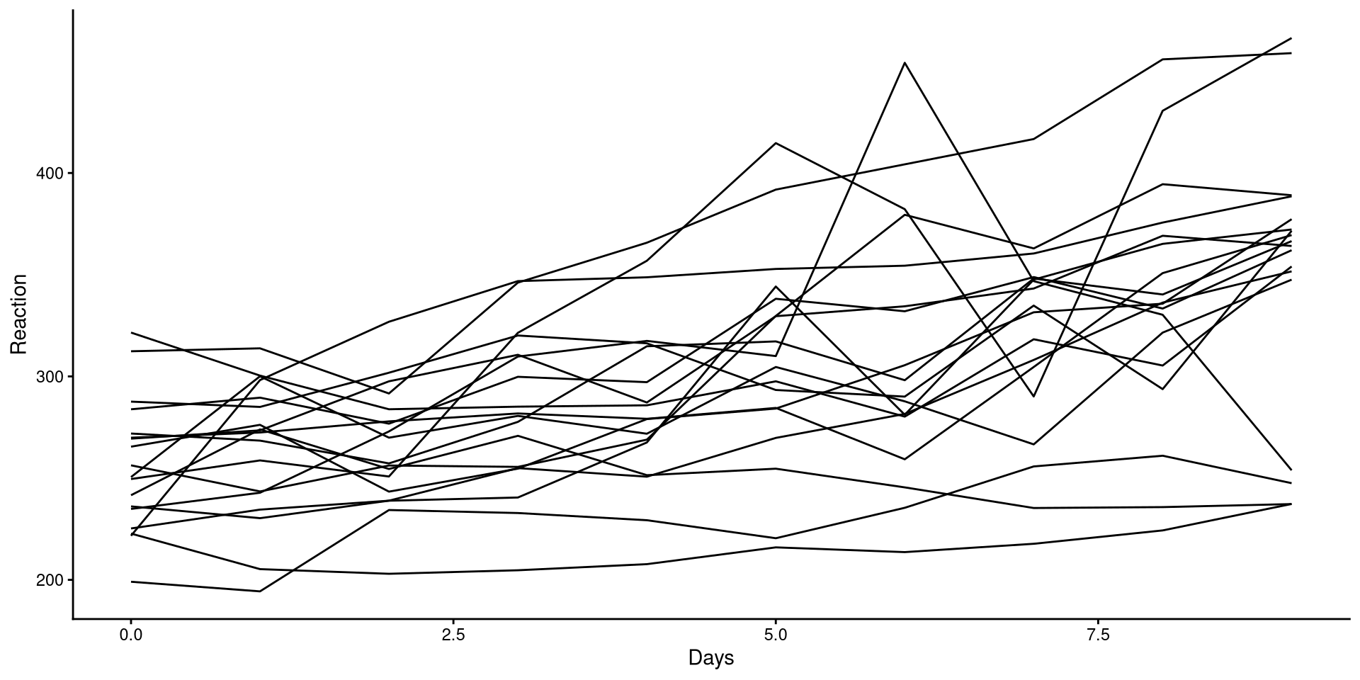
HLM is often employed in longitudinal designs, which is the case of these data. As such, we are often interested in the trend as time passes.
We can plot the trend of Reaction for each participant to get a sense of the general trend:
Although reaction times increase with higher sleep deprivation, we can see that the increase is not the same for all participants.
Fitting HLM with the lmerTest package
There are a couple of similarly name package to fit HLM models. I’ll just use lmerTest because it automatically includes significance tests for some of the results.
Linear mixed model fit by REML. t-tests use Satterthwaite's method [
lmerModLmerTest]
Formula: Reaction ~ (1 | Subject)
   Data: sleepstudy

REML criterion at convergence: 1904.3

Scaled residuals:
    Min      1Q  Median      3Q     Max
-2.4983 -0.5501 -0.1476  0.5123  3.3446

Random effects:
 Groups   Name        Variance Std.Dev.
 Subject  (Intercept) 1278     35.75
 Residual             1959     44.26
Number of obs: 180, groups:  Subject, 18

Fixed effects:
            Estimate Std. Error     df t value Pr(>|t|)
(Intercept)   298.51       9.05  17.00   32.98   <2e-16 ***
---
Signif. codes:  0 '***' 0.001 '**' 0.01 '*' 0.05 '.' 0.1 ' ' 1
We use the lmer() function from the lmerTest package. notice the formula:
Reaction ~ (1 | Subject)
Reaction is the DV, while the (1 | Subject) part tells R that we think that the participants will have different reaction times on average.
The (1 | Subject) part is also known as a random intercept, meaning that every Subject will have a different intercept.
HLM Results
You will notice that the summary has two sections
Linear mixed model fit by REML. t-tests use Satterthwaite's method [
lmerModLmerTest]
Formula: Reaction ~ (1 | Subject)
   Data: sleepstudy

REML criterion at convergence: 1904.3

Scaled residuals:
    Min      1Q  Median      3Q     Max
-2.4983 -0.5501 -0.1476  0.5123  3.3446

Random effects:
 Groups   Name        Variance Std.Dev.
 Subject  (Intercept) 1278     35.75
 Residual             1959     44.26
Number of obs: 180, groups:  Subject, 18

Fixed effects:
            Estimate Std. Error     df t value Pr(>|t|)
(Intercept)   298.51       9.05  17.00   32.98   <2e-16 ***
---
Signif. codes:  0 '***' 0.001 '**' 0.01 '*' 0.05 '.' 0.1 ' ' 1
Random Effects:
\(\hat{\psi} = 1278\): this is the variance of the mean reaction time across participants (between subject variance).
\(\hat{\theta} = 1959\): this is the variance of the residuals. Here it represents the within subject residuals and it is the variance that cannot be explained differences across people.
Fixed Effects:
\(\beta_0 = 298.51\): this is the same as the intercept in linear regression. Here it represents the average reaction time. The \(\hat{\psi}\) represents how much that varies between subjects.
Intraclass Correlation Coefficient
Because we are measuring the same individuals, we can expect measurement from the same individuals to be similar to each other. We can actually calculate how similar measurements from the same individuals are, and it’s done with the intraclass Correlation Coefficient (ICC).
The ICC is the amount of total variance in the outcome that is due to between group variation:
\[ ICC = \frac{\hat{\psi}}{\hat{\theta} + \hat{\psi}} = \frac{1278}{ 1959 + 1278} = .395 \]
This tells us the percentage of the variance in Reaction that is due to between subject difference (the higher the ICC, the more similar observations from the same subject will be). We can also use the icc() function from the performance to get the ICC:
Adding a Predictor
Linear mixed model fit by REML. t-tests use Satterthwaite's method [
lmerModLmerTest]
Formula: Reaction ~ (1 | Subject) + Days
   Data: sleepstudy

REML criterion at convergence: 1786.5

Scaled residuals:
    Min      1Q  Median      3Q     Max
-3.2257 -0.5529  0.0109  0.5188  4.2506

Random effects:
 Groups   Name        Variance Std.Dev.
 Subject  (Intercept) 1378.2   37.12
 Residual              960.5   30.99
Number of obs: 180, groups:  Subject, 18

Fixed effects:
            Estimate Std. Error       df t value Pr(>|t|)
(Intercept) 251.4051     9.7467  22.8102   25.79   <2e-16 ***
Days         10.4673     0.8042 161.0000   13.02   <2e-16 ***
---
Signif. codes:  0 '***' 0.001 '**' 0.01 '*' 0.05 '.' 0.1 ' ' 1

Correlation of Fixed Effects:
     (Intr)
Days -0.371
We can add predictors as we would with the lm() function by using the + symbol. If we scroll down to Fixed effects we see that now we have an additional parameter:
\(\beta_1 = 10.47\): This is the average increase in reaction time for each additional day of sleep deprivation.
Likelihood Ratio Test to Compare Models
We can also check whether adding Days as a predictors provides a significant improvement in predictions. Just as we have done previously, we use the anova() function:
Data: sleepstudy
Models:
HLM_mod: Reaction ~ (1 | Subject)
HLM_mod2: Reaction ~ (1 | Subject) + Days
         npar    AIC    BIC  logLik -2*log(L)  Chisq Df Pr(>Chisq)
HLM_mod     3 1916.5 1926.1 -955.27    1910.5
HLM_mod2    4 1802.1 1814.8 -897.04    1794.1 116.46  1  < 2.2e-16 ***
---
Signif. codes:  0 '***' 0.001 '**' 0.01 '*' 0.05 '.' 0.1 ' ' 1
On top of the likelihood ratio test (LRT), we also get the AIC and BIC, which are additional fit statistics. Lower AIC and BIC mean better fit. Similarly, a significant p-value indicates that the more complex model fits the data best.
Unsurprisingly, in every case, the model with Days as predictor fits the data best. Higher sleep deprivation does indeed increase reaction times.
References
Bates, D., Maechler, M., Bolker [aut, B., cre, Walker, S., Christensen, R. H. B., Singmann, H., Dai, B., Scheipl, F., Grothendieck, G., Green, P., Fox, J., Bauer, A., simulate.formula), P. N. K. (shared. copyright on, Tanaka, E., Jagan, M., & Boylan, R. D. (2025). Lme4: Linear Mixed-Effects Models using ’Eigen’ and S4.
Belenky, G., Wesensten, N. J., Thorne, D. R., Thomas, M. L., Sing, H. C., Redmond, D. P., Russo, M. B., & Balkin, T. J. (2003). Patterns of performance degradation and restoration during sleep restriction and subsequent recovery: A sleep dose-response study. Journal of Sleep Research, 12(1), 1–12. https://doi.org/10.1046/j.1365-2869.2003.00337.x
Kuznetsova, A., Brockhoff, P. B., Christensen, R. H. B., & Jensen, S. P. (2020). lmerTest: Tests in Linear Mixed Effects Models.
Lawrence, M. A. (2016). Ez: Easy Analysis and Visualization of Factorial Experiments.
Lüdecke, D., Aust, F., Crawley, S., Ben-Shachar, M. S., & Anderson, S. C. (2025). Ggeffects: Create Tidy Data Frames of Marginal Effects for ’ggplot’ from Model Outputs.
Schmidt, J. R., & Besner, D. (2008). The Stroop effect: Why proportion congruent has nothing to do with congruency and everything to do with contingency. Journal of Experimental Psychology: Learning, Memory, and Cognition, 34(3), 514–523. https://doi.org/10.1037/0278-7393.34.3.514
PSYC 6802 - Lab 14: Repeated Measures