Lab 13: Latent Variables
Fabio Setti
PSYC 6802 - Introduction to Psychology Statistics
Today’s Packages and Data 🤗
No new packages today!
We will be using the
pyschpackage for exploratory factor analysis (EFA).We will be using the
lavaanpackage for confirmatory factor analysis (CFA).
Today we will be looking at some data from Cox et al. (2008). As part of this study, the 200 participants completed the Positive and Negative Affect Schedule scale (PANAS) which is what we will focus on.
Some Preliminary Steps
Because the PANAS has already been analyzed, there is no need to run EFA. Here, we are running this example assuming that we just came up with the items and want to know how many latent factors the items may tap into.
We are only interested in the PANAS items, let’s subset the data so that it only includes those items. The paste0() function is epecially useful in this case; for example:
So if we want to select the columns named Panas1 to Panas20, we simply run:
If we plan on running both EFA and CFA, we should split our data randomly. The idea is that EFA serves as an exploratory analysis, while CFA serves to confirm your EFA findings on a new dataset.
Now we have two datasets, with 100 observations each. We will run EFA first and CFA later. The CFA will be informed by what we find in the EFA.
Determining Number of Factors
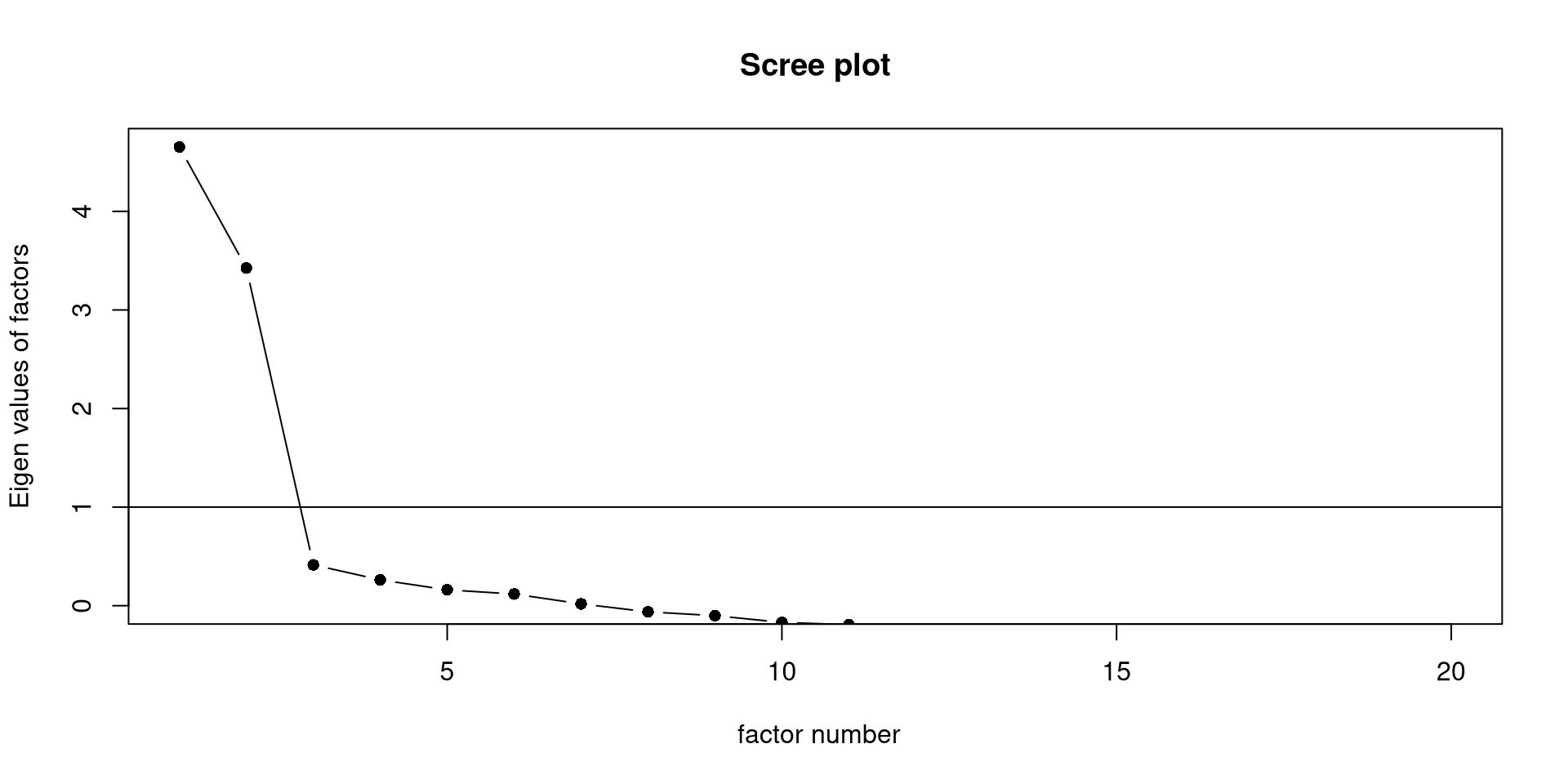
Let’s assume that we came up with some items, gave them to some people, and then want to know how many latent factors may be involved with those items. One way to determine the number of latent factors is using an elbow plot.
The scree() function from the psych package will create the elbow plot, also known as scree plot, for us.
The general wisdom is that there are as many meaningful latent factors as dots before the “elbow”. Here, I would say we definitely have 2 factors and maybe a third one (although unlikely).
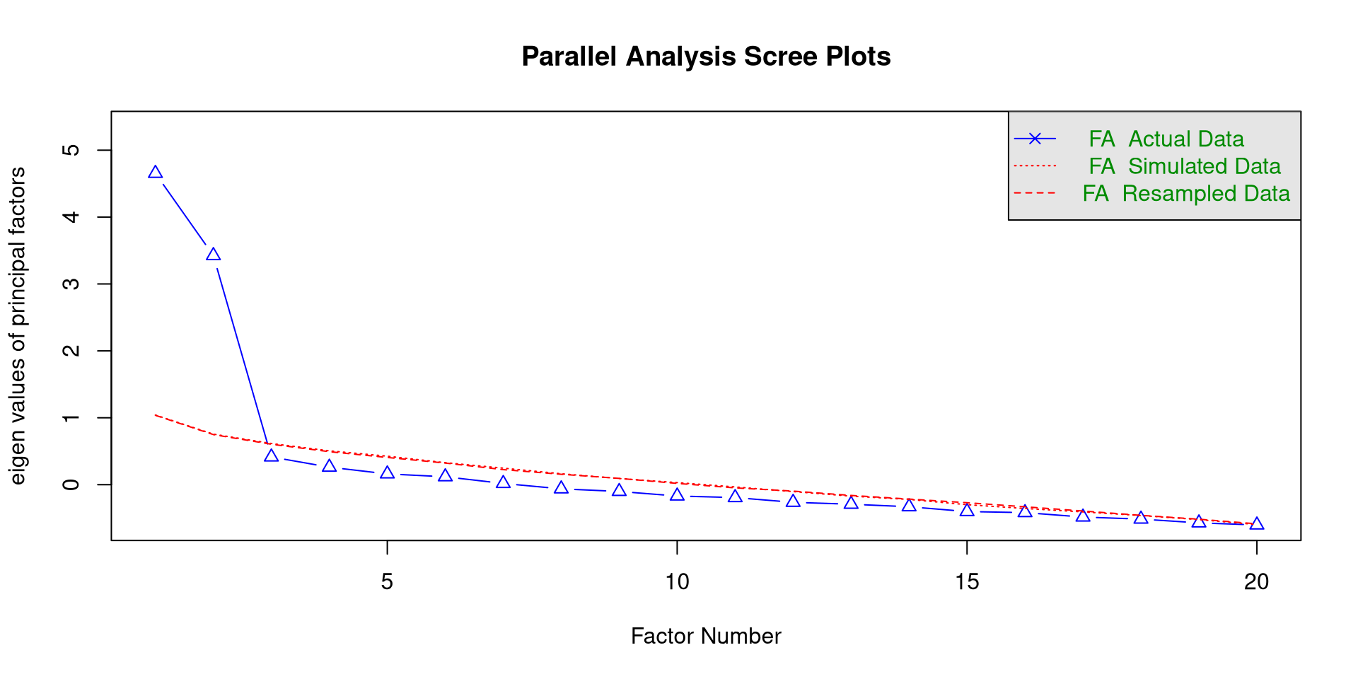
Parallel Analysis
Probably the most popular method for determining the number of meaningful latent factors is parallel analysis.
we can use the fa.parallel() function from the psych package to conduct a parallel analysis. If you are planmning on doing EFA, you need to specify fa = "fa" in the function.
The function will print the parallel analysis scree plot, which you should notice is different from the previous one.
We “retain” as many factors as triangles above the red line, so 2 factors. In general, this should be trusted more than the simple scree plot.
Exploratory Factor Analysis in R
we use the fa() function form the psych package to run an EFA in R.
Loadings:
        PA1    PA2
Panas1          0.609
Panas2   0.774
Panas3   0.329  0.435
Panas4   0.738
Panas5          0.652
Panas6   0.387
Panas7   0.711
Panas8   0.514
Panas9          0.766
Panas10         0.596
Panas11  0.543
Panas12         0.582
Panas13  0.401
Panas14         0.594
Panas15  0.742
Panas16         0.683
Panas17         0.702
Panas18  0.510
Panas19         0.743
Panas20  0.843

                 PA1   PA2
SS loadings    4.270 4.261
Proportion Var 0.214 0.213
Cumulative Var 0.214 0.427
nfactors =: here we specify the number of factors to extract. This number will depend on the results of the parallel analysis (or your theoretical knowledge).rotate =: here you specify the type of rotation."oblimin"is generally the suggested one.fm =: here you specify the factor extraction method."pa"stands for principal axis.
The cutoff = can be used inside the print() function the print the factor loadings but suppress the ones below a certain value. You can think of factor loadings as correlations between the item and the latent factor!
Do Our Results Align with theory?
We can find the PANAS here. On Page 2, some guidelines for scoring are given; do our EFA result align with the scoring guidelines?
Loadings:
        PA1    PA2
Panas1          0.609
Panas2   0.774
Panas3   0.329  0.435
Panas4   0.738
Panas5          0.652
Panas6   0.387
Panas7   0.711
Panas8   0.514
Panas9          0.766
Panas10         0.596
Panas11  0.543
Panas12         0.582
Panas13  0.401
Panas14         0.594
Panas15  0.742
Panas16         0.683
Panas17         0.702
Panas18  0.510
Panas19         0.743
Panas20  0.843

                 PA1   PA2
SS loadings    4.270 4.261
Proportion Var 0.214 0.213
Cumulative Var 0.214 0.427The guidelines tell us that:
Positive affect (PA): items 1, 3, 5, 9, 10, 12, 14, 16, 17, and 19.
Negative affect (NA): items 2, 4, 6, 7, 8, 11, 13, 15, 18, and 20.
In our sample, PA1 has strong loadings for almost all the negative affect items, while PA2 has strong loadings for almost all the positive affect items. Thus, we can deduce that:
Notably, item 3 does not seem to work super well in our sample.
Defining the CFA Model
Once again, I am assuming that we are working with a completely new scale and that we just run EFA on a part of the data. Now we need to confirm our findings on the rest of the data with CFA.
We use lavaan to run the CFA. When with latent factors, we use the =~ operator to define them:
This is the CFA model that we will run in lavaan. Notice that, for each item, we specify a loading only for the factor that had the highest loadings in the EFA table (although I am oversimplifying the process).
With the model above we are making a clear theoretical statement:
“items 1, 3, 5, 9, 10, 12, 14, 16, 17, and 19 only measure positive affect, while the other items only measure negative affect”
CFA allows us to test how well the data conforms to our theoretical statement. If the data conforms to our theory, then we likely have a good theory. If the data does not support our theory, then we are likely missing something.
Confirmatory Factor Analysis in R
We can use the sem() function to run the CFA and standardizedSolution() to get some summaries:
            lhs op          rhs est.std    se      z pvalue ci.lower ci.upper
1  Positive_aff =~       Panas1   0.450 0.084  5.331  0.000    0.285    0.615
2  Positive_aff =~       Panas3   0.380 0.090  4.220  0.000    0.204    0.557
3  Positive_aff =~       Panas5   0.572 0.072  7.949  0.000    0.431    0.714
4  Positive_aff =~       Panas9   0.837 0.036 23.140  0.000    0.766    0.908
5  Positive_aff =~      Panas10   0.759 0.048 15.871  0.000    0.665    0.852
6  Positive_aff =~      Panas12   0.694 0.057 12.180  0.000    0.582    0.805
7  Positive_aff =~      Panas14   0.691 0.057 12.041  0.000    0.578    0.803
8  Positive_aff =~      Panas16   0.801 0.042 19.253  0.000    0.719    0.882
9  Positive_aff =~      Panas17   0.634 0.065  9.786  0.000    0.507    0.761
10 Positive_aff =~      Panas19   0.815 0.040 20.618  0.000    0.737    0.892
11 Negative_aff =~       Panas2   0.641 0.065  9.866  0.000    0.514    0.769
12 Negative_aff =~       Panas4   0.673 0.061 11.026  0.000    0.553    0.792
13 Negative_aff =~       Panas6   0.221 0.101  2.198  0.028    0.024    0.418
14 Negative_aff =~       Panas7   0.804 0.043 18.740  0.000    0.720    0.888
15 Negative_aff =~       Panas8   0.381 0.091  4.178  0.000    0.202    0.559
16 Negative_aff =~      Panas11   0.591 0.071  8.327  0.000    0.452    0.730
17 Negative_aff =~      Panas13   0.517 0.079  6.530  0.000    0.361    0.672
18 Negative_aff =~      Panas15   0.814 0.041 19.657  0.000    0.733    0.895
19 Negative_aff =~      Panas18   0.455 0.085  5.350  0.000    0.288    0.621
20 Negative_aff =~      Panas20   0.831 0.039 21.272  0.000    0.754    0.907
21       Panas1 ~~       Panas1   0.798 0.076 10.502  0.000    0.649    0.946
22       Panas3 ~~       Panas3   0.855 0.069 12.477  0.000    0.721    0.990
23       Panas5 ~~       Panas5   0.672 0.082  8.155  0.000    0.511    0.834
24       Panas9 ~~       Panas9   0.300 0.061  4.954  0.000    0.181    0.418
25      Panas10 ~~      Panas10   0.424 0.073  5.850  0.000    0.282    0.567
26      Panas12 ~~      Panas12   0.519 0.079  6.567  0.000    0.364    0.674
27      Panas14 ~~      Panas14   0.523 0.079  6.602  0.000    0.368    0.678
28      Panas16 ~~      Panas16   0.359 0.067  5.387  0.000    0.228    0.489
29      Panas17 ~~      Panas17   0.599 0.082  7.295  0.000    0.438    0.759
30      Panas19 ~~      Panas19   0.336 0.064  5.227  0.000    0.210    0.463
31       Panas2 ~~       Panas2   0.589 0.083  7.067  0.000    0.426    0.752
32       Panas4 ~~       Panas4   0.548 0.082  6.675  0.000    0.387    0.708
33       Panas6 ~~       Panas6   0.951 0.044 21.375  0.000    0.864    1.038
34       Panas7 ~~       Panas7   0.354 0.069  5.142  0.000    0.219    0.489
35       Panas8 ~~       Panas8   0.855 0.069 12.327  0.000    0.719    0.991
36      Panas11 ~~      Panas11   0.651 0.084  7.750  0.000    0.486    0.815
37      Panas13 ~~      Panas13   0.733 0.082  8.974  0.000    0.573    0.893
38      Panas15 ~~      Panas15   0.338 0.067  5.009  0.000    0.205    0.470
39      Panas18 ~~      Panas18   0.793 0.077 10.260  0.000    0.642    0.945
40      Panas20 ~~      Panas20   0.310 0.065  4.783  0.000    0.183    0.437
41 Positive_aff ~~ Positive_aff   1.000 0.000     NA     NA    1.000    1.000
42 Negative_aff ~~ Negative_aff   1.000 0.000     NA     NA    1.000    1.000
43 Positive_aff ~~ Negative_aff 0.022 0.110 0.197 0.844 -0.194 0.238- The rows with
=~are the factor loadings and their value is underest.std.
- The rows with
~~are variances and covariances (explaining this requires a whole lecture in of itself, so can’t provide much more context). The only thing that I will note is that the last rowPositive_aff ~~ Negative_affis the correlation between the two latent factors.
Assessing Model Fit
As previously mentioned that big advantage of CFA is that it allows to test our model by allowing us to assess how well the model fits the data. There are MANY measures model fit indices, but we will limit ourselves to the most popular ones:
- the \(\chi^2\) is generally the harshest fit measure. In theory, if it is significant, it indicates the model does not fit the data well. In practice it is almost always significant, so RMSEA, SRMR and CFI are generally more popular.
- \(RMSEA \leq .05\) is considered good. Here we have \(RMSEA = .12\), not good ❌
- \(SRMR \leq .08\) is considered good. Here we have \(SRMR = .11\), not good ❌
- \(CFI \geq .95\) is considered good. Here we have \(CFI = .76\), really not good ❌
So, our data does not support this structure of the PANAS. Is the PANAS bad? It’s more likely that our CFA sample size (\(N = 100\)) is a bit too small to make any real conclusions.
References
Cox, C. R., Arndt, J., Pyszczynski, T., Greenberg, J., Abdollahi, A., & Solomon, S. (2008). Terror management and adults’ attachment to their parents: The safe haven remains. Journal of Personality and Social Psychology, 94(4), 696–717. https://doi.org/10.1037/0022-3514.94.4.696
PSYC 6802 - Lab 13: Latent Variables