Lab 1: Introduction to R

Fabio Setti

PSYC 6802 - Introduction to Psychology Statistics

R and RStudio?

To start, it’s good to point out that R and RStudio are two different things

RStudio:

What is R?

R (https://www.r-project.org/about.html) is a programming language originally designed for statistical computing and data visualization.

Thanks to the contribution of many users, nowadays R is quite similar to python (https://www.python.org) in what it allows you to do.

There exist many programming languages and some do something better than others.

R works pretty well for data analysis and visualization and that’s why we use it 🤷

What is RStudio?

Whereas R is a programming language, RStudio is an integrated development environment (IDE…a what? 😕)

An IDE is software that facilitates writing code in general. Although RStudio was developed with R in mind, it also supports many other programming languages (e.g., Python, Javascript, C…)

Likewise, you do not need RStudio to use R. However, RStudio is by far the best IDE for coding in R and it makes the process much more efficient!

The people who make RStudio (https://posit.co/download/rstudio-desktop) have no affiliation with the people who make R as far as I know.

Coding

To use R properly you will have to learn how to code (which may sound a bit scary 😟). Coding is like learning a foreign language: There is grammar and there is a logic to how you construct sentences. The exact same is true for programming languages. There is a lot I could say here, but just some advice:

Errors and Mistakes: Your code (my code too!) will almost never work perfectly the first time around. Do not get frustrated; understand why your code does not work. Making mistakes over and over and fixing them is how your learn.

Understand Your Code: Do not copy and paste code without understanding what it does. This may work for some of the assignments in this course, but it will eventually lead to huge mistakes when you are doing research on your own.

Taking Shortcuts: There are many shortcuts you can take to write code (e.g., chatGPT). I strongly discourage using AI assistance to write code if you are new to coding. AI code may be wrong (or it may not be what you want), and you first need to develop the knowledge to know when and why code is wrong.

If you have code problems (and I am not around to help), I recommend Googling your question and looking for other humans who have answered it (usually on https://stackoverflow.com)

RStudio: What Am I looking at?

The RStudio interface is divided into 4 panes:

Source (top-left): This pane is where we will do most of our work. Here is were you can edit and run your code files (scripts).

Environment (top-right): This is where you can find the objects that are present in the current R session.

Console (bottom-left): The console is actually R by itself (the R console) and it is how RStudio runs R. You will find output, messages, and warnings here.*

Viewer (bottom-right): This is a bit of a catch-all pane. Here, you will find plots, installed packages, help for functions, and your computer folders (under files)

(You can customize where your panes are. I usually swap the position of the console and environment)

More about the “Console”

You can actually write and run code directly in the console, but you cannot save your code (which you should always do!). When you run your code from the Source pane, RStudio sends it to the console to be interpreted. All computer code is just plain text; what you need to run code of a certain computer language is to have something that interprets it and runs it. The R console is what interprets and runs your code (Hence why you need to have R on your computer to use R in RStudio)

Creating an R Script

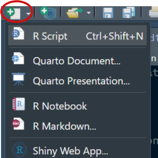
Before we can do any coding, we need to open a new R script! You can open a new R script by following the steps in the image on the right, or by using pressing Crtl + Shift + N (Windows) or Cmd + Shift + N.

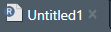
A tab named “Untitled1” will appear in your source pane. This is where we are going to write code for today!

As any other file, you can later save this file anywhere on your computer. It will have the .R extension.

👉 Save the file and name it “Lab_1_code” 👈

Running Code and Mathematical Operations

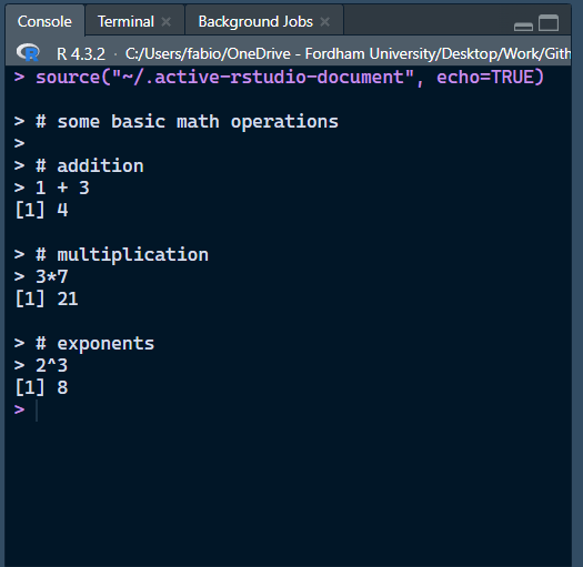
R can perform just about any mathematical operation. At the same time, let’s see how to run some code:

In RStudio, you can either run one or more line of code at once, or run the whole R script file at once.

One or more lines: highlight the lines that you want to run and press Ctrl + Enter (Windows) or Cmd + Return (Mac)

Entire Script: press Ctrl + Shift + Enter (Windows) or Cmd + Shift + Return (Mac).

The 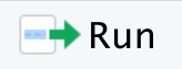button will also run the next runnable line of code with respect to your cursor.

👉 Copy the code chunk on the right into your R script and try running the full script. 👈

# some basic math operations

# addition
1 + 3

# multiplication
3*7

# exponents
2^3

Output

You will see your code with output appear in the console.

Output is indicated by “[n]”, where n represents the line of the output.

Here we only have one line for output each of our inputs (the 3 math operations), but you can have more lines.

The # sign represents comments. R will not run commented lines. Comments are good for explaining code to other people reading your code, and more importantly…to the future you!

A Note on how R Interprets Code

R “reads” code until it find the end of a statement (code that produces output), and then expects the following statement to appear on a new line.

For example:

# The line below is a statement and will produce output

(4 +5)*2

[1] 18

However:

# The this will not run (2 statements on the same line)

(4 + 5)*2  6+6

Error in parse(text = input): <text>:3:12: unexpected numeric constant
2: 
3: (4 + 5)*2  6
              ^

Spacing among elements of a statement is irrelevant, but it is good practice to be reasonable and consistent.

# This is not good practice, but it will run.

( 4 +
  5 )*   2

[1] 18

6  +
   6

[1] 12

Operators

Operators are symbols that tell R to perform certain actions. Aside from the math operations, the : operator is a bit unique to R.

Operator	Description
`+`	addition
`-`	subtraction
`*`	multiplication
`/`	division
`^`	exponentiation
`x:y`	sequence from x to y

Although it may no appear so, : turns out to be very convenient in many cases

3:10

[1]  3  4  5  6  7  8  9 10

There exist other operators and logical operators as well, but I will talk about them as they come up.

If you are curious, you can find a more comprehensive list of R operators here

Objects

Just as many other programming languages, R is object-oriented. You can think of objects as containers where information is stored (very important concept to remember).

To create an object in R, you use “<” + “-”, known as the assignment operator:

# This means x "is" (4 +5)*2. you can name objects whatever you want but the name cannot begin with a number or include special characters (?, !, etc...). 

x <- (4 +5)*2

The keyboard shortcut for the assignment operator is alt + - (Win) or Option + - (Mac).

No output is produced. However, you will now see the x object appear in your environment!

R now knows that whenever you write x in your code, you mean 18.

x + 3

[1] 21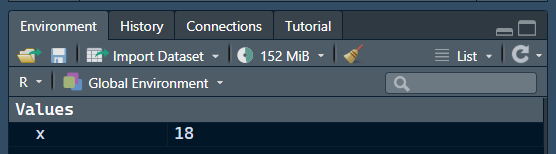

Types of Objects and Dimensions

Just like there are different types of containers (boxes, drawers, fridges, etc…), there are different types of R objects!

The x object that we just created is a numeric vector (type of object) of length 1 🤔

A vector is a one-dimensional collection of elements. To create a vector with more than one element we can do the following:

# `c()` is a function (more on functions later), and it stands for "concatenate". The `c()` binds elements together.`c()` is probably the most used R function. `y` will be a vector of length 4.

y <- c(1, 5, 7, 9)

# math operations can be applied to vectors!

y - 3

[1] -2  2  4  6

The concept of dimensions will become clearer later. In the meantime, can you think of some objects that may have more than 1 dimension? 🤓

Character Objects

So far we have only dealt with numbers, but character objects also come up a lot:

# Characters need to be enclosed within "" or ''. This is so that R knows you are not referring to an object ("x" is a character, just x is expected to be an object in your environment)
x <- "Hello"
y <- c("hello", "world", "what time is it?")

you cannot apply any math operations to character objects

# this will not run
y - 3

Error in y - 3: non-numeric argument to binary operator

Also note that you can create character objects/vectors that have numbers in them, but you will not be able to apply math operations to them:

x <- c("2", "23", "4")
# this will not run
x - 6

Error in x - 6: non-numeric argument to binary operator

Functions

A function is something that takes one or more objects as input and produces some output.

R interprets anything that stars with letters and is followed by a ( as a function, after which it executes the function until the next ).

x <- c(2,10, 4, 11, 12, 6)
# `sum()` is a function; x is the input and the sum of the elements of x is the output
sum(x)

[1] 45

R is case sensitive, so Sum() will not work:

# there is no `Sum()` function, only `sum()`
Sum(x)

Error in Sum(x): could not find function "Sum"

Functions also have arguments, that allow you to tweak what the function does. Here decreasing = is an argument of the sort() function:

# `Sort()`, by default, sorts vectors from smallest to largest (or in alphabetical order if you give it a character!)
# Here, we use "decreasing = TRUE" to sort from largest to smallest. 

sort(x, decreasing = TRUE)

[1] 12 11 10  6  4  2

Functions are at the core of anything we do in R. We will learn about many more functions as they come up. If you want to get a flavor of some basic R functions, you can find a list here.

The Help Menu

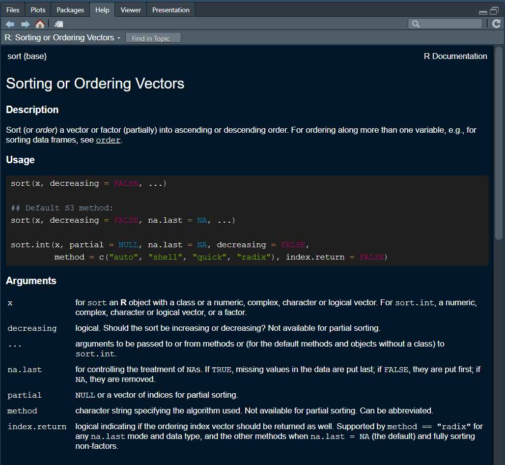
Let’s say I ask Google for an R function that sorts vectors and I find the sort() function!…But how do I know about its arguments? How do I know whether it sorts in ascending or descending order by default? How do I know that the function does what I need? 🤔

This is where RSstudio’s help menu comes to the rescue! 😀

# run the empty function with "?" in front of it to open it's help menu
?sort()
# Alternatively you can also highlight or hover over the function (just the function, not the "()") and press F1.

Description: Brief description of that the function does.

Usage: Shows default values of arguments (i.e., “decreasing” is set to FALSE unless you say otherwise).

Arguments: all the function arguments and what each one does!

There’s much more going on here, but notice the {base} after the name of the function. That is the package the function comes from 🧐

Packages

Usually, the base R functions are not enough for most of the tasks that one needs to accomplish in R. Often people have to create their own custom functions.

A package is simply a collection of functions that other users make for everyone out of the kindness of their heart 🤗

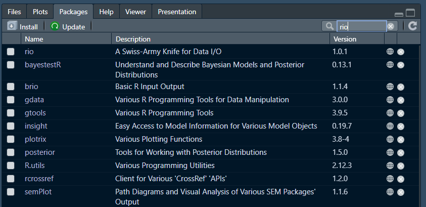
Let’s install a package that makes opening data in R very smooth, the rio package (Becker et al., 2024):

# This is how you install packages from CRAN (explained below)
install.packages("rio")

The install.packages() function installs packages from the comprehensive R archive network (CRAN). Among other things, CRAN maintains a library of packages made by users.

The process to get a package on CRAN is a bit lengthy (and sometimes packages get removed), so some people just upload their packages to Github.

To see all of the packages installed in your RStudio, you can navigate to your viewer pane and select “packages”.

Reading files: Working Directories

We want to open the World_happiness_2024.csv data set with the import() function from the rio package. First we download the data (click here). Then we load the rio package:

# to load the functions from a package you need to run the `library(package)` function first
library(rio)

# rio also suggests to add a few extra packages, so also run the line below. It is the case that packages have functions that use functions from other packages to run, hence why rio suggests to also install other packages here
install_formats()

Now, we need to tell R how to find the World_happiness_2024.csv file. Here are a couple of ways of doing this:

Either you use the absolute file path (i.e., a unique address that identifies the location of all files on your computer)

Change your working directory (WD; the default folder where RStudio saves/looks for files) to where the data is (or move the data to your current WD). Your current WD is always displayed at the top of the R console pane next to the R version number.

I will show one quick way of dealing with working directories, which I don’t consider best. My preferred way by far is using RStudio projects, which I may talk about at some point.

Setting Working Directory

You can get your current working directory by running the getwd() function. This is where R currently expects to find files.

# `getwd()` is actually a function that take no input!
getwd()

[1] "C:/Users/fabio/Dropbox/Work/Github repos/Fabio-Setti/static/PSYC6802"

I’ll change my current working directory to my Desktop with the setwd() function. This function takes the path to a location on your computer as input. For the Desktop:

setwd("~/Desktop") on Mac
setwd("C:/Users/fabio/Desktop") on Windows.

# on windows, change "fabio" to your windows username
setwd("C:/Users/fabio/OneDrive/Desktop")

Everyone will have something different here

For Mac, make sure that files you want to open are stored on your computer and not on the cloud (R does not see files stored on the cloud).
OneDrive is really annoying on Windows and puts itself before my Desktop (😤). If you have OneDrive, this will likely happen to you too.

Afterwards, move the World_happiness_2024.csv to your Desktop (which should now be your WD)

Loading Data and Looking at it

Now that our working directory is (hopefully) sorted out, we can use the import() function from rio to load our data. Data needs to be saved as a new object, so we use <- to name it:

# I name the data `dat`. an object named `dat` will appear in your environment
dat <- import("World_happiness_2024.csv")

This is data from the 2024 world happiness report. The str() function can be used to get a lot of information about objects:

# you can also click on the `dat` object in your environment to open it in the data viewer mode
str(dat)

'data.frame':   140 obs. of  9 variables:
 $ Country_name           : chr  "Finland" "Denmark" "Iceland" "Sweden" ...
 $ Region                 : chr  "Western Europe" "Western Europe" "Western Europe" "Western Europe" ...
 $ Happiness_score        : num  7.74 7.58 7.53 7.34 7.34 ...
 $ Log_GDP                : num  1.84 1.91 1.88 1.88 1.8 ...
 $ Social_support         : num  1.57 1.52 1.62 1.5 1.51 ...
 $ Healthy_life_expectancy: num  0.695 0.699 0.718 0.724 0.74 0.706 0.704 0.708 0.747 0.692 ...
 $ Freedom                : num  0.859 0.823 0.819 0.838 0.641 0.725 0.835 0.801 0.759 0.756 ...
 $ Generosity             : num  0.142 0.204 0.258 0.221 0.153 0.247 0.224 0.146 0.173 0.225 ...
 $ Corruption             : num  0.454 0.452 0.818 0.476 0.807 0.628 0.516 0.568 0.502 0.677 ...

`data.frame` Objects

Although this information was given to us by the str() function, it is generally useful to first figure out what type of object we are dealing with:

# When things don't work, check that you are using the right object class (e.g., some functions want data.frame objects and not matrix objects, which are pretty similar but not the same)
class(dat)

[1] "data.frame"

the dat object is a data.frame. We will come across other type of objects eventually, but here is a list of common ones.

For data.frame objects you can use the $ operator to refer to columns.

# get the mean of the `Happiness_score` column 
mean(dat$Happiness_score)

[1] 5.530893

Let’s also count how many countries are in each Region. The table() function is quite useful for counting categories

table(dat$Region)


        Africa           Asia      Caribbean Eastern Europe   Middele East 
            40             22              2             23             11 
 North America        Oceania  South America Western Europe 
             8              2             11             21

Back to Dimensions: Subsetting

You may have realized that data.frame objects, unlike vectors, have 2 dimensions (2D), rows and columns.

Now, If objects are containers for information, then there must be a way to extract only some of the information stored in those containers 🧐 This is called subsetting (or indexing, depends on the context).

You can subset 2D objects by referring to the indices of their dimensions in this way object_name[row number, column number]:

# Select the element of [row 1, column 1] of the `dat` object
dat[1,1]

[1] "Finland"

# You can select the entire 2nd row of the "dat" object. If you leave a dimension empty when subsetting, it means "all of this dimension".
dat[2,]

  Country_name         Region Happiness_score Log_GDP Social_support
2      Denmark Western Europe           7.583   1.908           1.52
  Healthy_life_expectancy Freedom Generosity Corruption
2                   0.699   0.823      0.204      0.452

More Subsetting Examples

You can modify specific elements like so:

# You can remove (or substitute!) elements in this way. The "dat_2" object will be "dat" without the first row. `nrow()` counts the rows of a 2D object. 
dat_2 <- dat[-1,]
nrow(dat_2)

[1] 139

You can also select non-adjacent elements:

# You refer to non-adjacent columns/rows through the `c()` function. This selects element 1,4,6 of column 6 of the `dat` object
dat[c(1,4,6) ,6]

[1] 0.695 0.724 0.706

…and the 1D case follows a similar logic:

# To subset 1D elements, you simply do this. Here, I get the 5th element of the `x` object
x <- c(3, 2, 5, 10, 23)
x[5]

[1] 23

Is all of this worth Your Time?

I often get students telling me that “they prefer SPSS” (my nemesis 🙃). Normally, I would go on a 20 minutes rant about this, but some like-minded people have done that in this pretty funny reddit post

Some other reasons for adopting R:

Free: R is free and will always be. SPSS and the like charge ridiculous amounts for licenses. (support free stuff, knowledge should be accessible)

Reproducibility: Ever heard of the replication crisis? R makes it much easier to share code and analyses so that results can be reproduced and checked thoroughly.

Open source: There are thousands of people constantly working on R packages, expanding R’s features every day.

Flexibility: R can do just about anything you need. Whereas if you use other software like SPSS, you will likely hit a wall because you need to do something that the software does not allow you to do.

Learning R may be hard at first, but please believe me when I say that it will be well worth it in the end 🤗

But wait! One last thing 🫣

Reporting With Quarto!

What is Quarto?

Quarto is an “open-source scientific and technical publishing system”. As mentioned on their main page, with quarto, you can:

Create reports that seamlessly integrate plain text and R code (even python and Julia)

Create documents and easily publish them online for everyone to access.

Publish reproducible, production quality articles, presentations (e.g., these slides!), dashboards, websites, blogs, and books in HTML, PDF, MS Word, ePub, and more.

In this course, you will use quarto to produce PDF reports for your lab activities and homework assignments.

Overall I am a big fan of quarto because it fosters accessibility, reproducibility, and transparency 😀

Setting Up Quarto To Create PDFs

Before we can create PDFs with quarto, there are 2 important steps that you need to follow:

Step 1:

First, you need to install the rmarkdown package (Allaire et al., 2024).

install.packages("rmarkdown")

R Markdown used to be the main way (and may still be) of creating reports in R. However, the RStudio folks have decided to move to quarto, and it will likely become more popular than R Markdown in the near future.

Step 2:

In general, most of the nice PDFs you see are created with LaTeX. The last thing that we need is to install a LaTeX interpreter (kinda like needing R to run R code!).

To install a LaTeX interpreter that quarto likes, go to the top of your screen and click tools → terminal → new terminal

A window named “terminal” will appear next to the R console. Go to the “terminal” window, type the following line :

quarto install tinytex

and the press Enter (Win) or Return (Mac)

Opening a quarto file

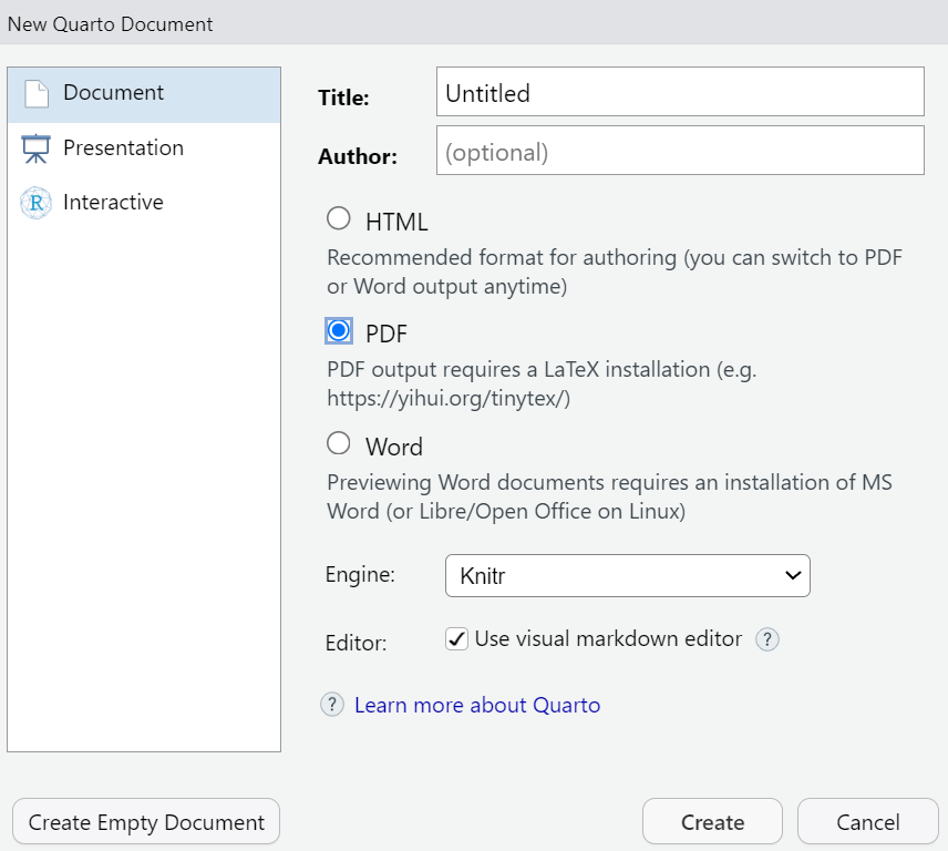
quarto files have the .qmd extension. We can open a .qmd file by clicking file → new file → quarto document. You should see the window on right appear. Make sure you select PDF.

Note the Use visual markdown editor check-box. Once you create the document you will have the option to switch between the visual and source editor:

Source editor: The file will look like a plain code file. (I much prefer to use this)

Visual editor: The file will look more like a word doc and you will have some point-and-click shortcuts to edit text. This is more user friendly, although it can get a bit clunky.

Click on Create to create a .qmd document, which will already have some instructions in it.

Creating a PDF

Now you can click on Render at the top of the document; you will be asked to save the .qmd file. After you do, you will see a .pdf file appear where you saved your .qmd file.

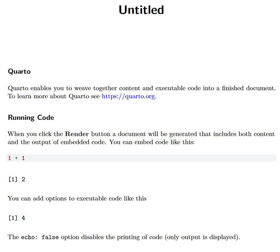
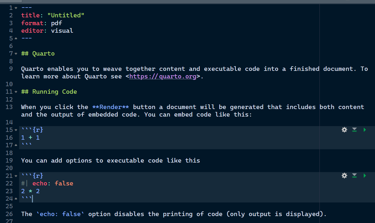
This is what the .qmd file looks like from the source editor view:

The PDF file output:

The YAML Header

The fist thing that we see in the .qmd file is the are some lines enclosed between two ---. That is a YAML header. The YAML header simply gives quarto some instruction to follow once you click the “Render” button.

default YAML header:

---
title: "Untitled"
format: pdf
editor: visual
---

Add author to YAML header and change title:

---
title: "Example"
author: Your name
format: pdf
editor: visual
---

Try to make the changes in the second code block and render the PDF again!

For this course, I don’t expect you to make any changes to the YAML header beyond modifying the title and adding your name as the author. Here is a comprehensive list of all the YAML options that exists for PDF documents in quarto.

Plain Text and Code Chunks

.qmd files have two main parts plain text and code chunks

Plain text

Any text outside code chunks is considered plain text. In the template .qmd file “Quarto enables you to…document.” is plain text. When creating PDF files from .qmd files, plain text accepts both Markdown (see here) and LaTeX syntax.

In this course, LaTeX syntax will only come up if you want to write Greek letters or math symbols (see here)

Anything in plain text between $ signs is interpreted as LaTeX math. So, $\beta$ will look like $\beta$, or $\sqrt{x}$ will look like $\sqrt{x}$ (LaTeX looks nice, so give it a try 🫣)

Code chunks

Code chunks are anything that is enclosed between ```{r} and ```

```{r}
1+1
```

[1] 2

You can create a new code chunk with Ctrl + Alt + I (Windows) or Cmd + Option + I (Mac).

Code chunks can be run in many ways, one of them being the green arrow at their top right.

You can also modify how the chunks behave when rendered with chunk options (e.g., your advisor does not know R, so you can hide the code and just show the output).

More about Code Chunks

1. When quarto renders a .qmd file, it will run R chunks in order, one by one. This means that your code should work in sequence from the first chunk to the last chunk. For example:

If you had this chunk

```{r}
x + 5
```

Followed later by this chunk first

```{r}
x <- 4
```

Your document will not render because in the x + 5 part, R does not know what x is yet 🧐 I suggest that before you try rendering your document, you run rm(list=ls()) to clear your environment and check that your code runs from start to finish!

2. You only need to install packages once. Do not leave install.packages() functions in your code chunks when trying to render; that will also likely cause issues.

3. You can make your PDF documents look much better by modifying chunk options (e.g., hiding messages and warnings by using #| message: false and #| warning: false in your chunks). You really don’t have to do this, but I would really appreciate if you spent a tad bit more time improving how you PDFs look (makes grading homework easier 🥺)

References

Allaire, J. J., Xie [aut, Y., cre, Dervieux, C., McPherson, J., Luraschi, J., Ushey, K., Atkins, A., Wickham, H., Cheng, J., Chang, W., Iannone, R., Dunning, A., filter), A. Y. (cph:. N. sections L., Schloerke, B., Sievert, C., Ryan, D., Aust, F., Allen, J., … filter), A. K. (pagebreak. L. (2024). Rmarkdown: Dynamic Documents for R (Version 2.29) [Computer software]. https://cran.r-project.org/web/packages/rmarkdown/index.html

Becker, J., Chan, C., Schoch, D., Chan, G. C., Leeper, T. J., Gandrud, C., MacDonald, A., Zahn, I., Stadlmann, S., Williamson, R., Kennedy, P., Price, R., Davis, T. L., Day, N., Denney, B., Bokov, A., & Gruson, H. (2024). Rio: A Swiss-Army Knife for Data I/O (Version 1.2.3) [Computer software]. https://cran.r-project.org/web/packages/rio/index.html